Author Archive Admin

Net Asset Value (NAV)


Net Asset Value (NAV): A Detailed Explanation

Net Asset Value (NAV) is a key financial metric used to measure the value of an investment fund, such as a mutual fund, exchange-traded fund (ETF), or hedge fund. NAV represents the per-share value of a fund’s assets, minus its liabilities, and is often used to determine the price at which investors buy and sell shares in the fund. It provides investors with an understanding of the underlying value of the assets held by the fund.

NAV is particularly important in the context of investment funds, as it directly reflects the current value of the fund’s holdings and is essential for calculating the performance of the fund over time.


1. Formula for Net Asset Value (NAV):

The formula for calculating NAV is as follows:


NAV=Total AssetsTotal LiabilitiesOutstanding Shares\text{NAV} = \frac{\text{Total Assets} – \text{Total Liabilities}}{\text{Outstanding Shares}}


Where:

  • Total Assets: This includes the market value of all the assets held by the fund, such as stocks, bonds, cash, and any other investments.
  • Total Liabilities: This represents any debts or obligations the fund has, such as pending expenses, management fees, and any other liabilities.
  • Outstanding Shares: This refers to the total number of shares of the fund that are currently owned by all investors.


2. Steps in Calculating NAV:

To understand how NAV is calculated, consider the following steps:

a. Calculate Total Assets:
  • Add up the value of all the securities and assets the fund owns. This includes the value of stocks, bonds, real estate, cash, or any other investments.
  • For example, if the fund holds stocks worth $10 million, bonds worth $5 million, and cash of $1 million, the total assets would be:

Total Assets=10million+5million+1million=16million\text{Total Assets} = 10 \, \text{million} + 5 \, \text{million} + 1 \, \text{million} = 16 \, \text{million}


b. Calculate Total Liabilities:
  • This includes all the debts and obligations the fund owes. Liabilities could consist of unpaid fees, loans, or other financial obligations.
  • For example, if the fund has liabilities of $2 million, then:


Total Liabilities=2million\text{Total Liabilities} = 2 \, \text{million}


c. Calculate the Outstanding Shares:
  • This refers to the total number of shares that have been issued by the fund. For example, if the fund has issued 1 million shares:

Outstanding Shares=1,000,000\text{Outstanding Shares} = 1,000,000


d. Apply the NAV Formula:
  • Now, you can calculate the NAV by subtracting liabilities from assets and then dividing by the number of outstanding shares:


NAV=16million2million1,000,000=14million1,000,000=14\text{NAV} = \frac{16 \, \text{million} – 2 \, \text{million}}{1,000,000} = \frac{14 \, \text{million}}{1,000,000} = 14


So, the NAV of the fund is $14 per share.


3. Why is NAV Important?

NAV plays a crucial role in the following ways:

a. Valuation of Investment Funds:
  • NAV gives investors an accurate and updated valuation of a mutual fund, ETF, or other pooled investment vehicles. It reflects the current market value of the assets held by the fund.
  • It is essential for determining how much an investor would receive per share if they decide to redeem or sell their shares in the fund.
b. Fund Performance:
  • NAV is used to track the performance of an investment fund. If the NAV is increasing, it generally indicates that the value of the fund’s assets is rising, which is a positive sign for investors.
  • Conversely, if the NAV decreases, it could suggest that the value of the fund’s investments is declining, which may be a signal for concern.
c. Purchase and Redemption Price:
  • NAV is the price at which mutual fund shares are bought and sold. When you invest in a mutual fund, you are essentially buying shares at the NAV price. Similarly, when you redeem your shares, you are selling them at the NAV price.
  • The NAV is calculated at the end of each trading day, and mutual funds use this figure to process buy or sell orders for their investors.


4. NAV and Mutual Funds:

In mutual funds, the NAV is calculated once a day at the close of the market, usually after the market closes (e.g., 4:00 PM ET in the United States). The NAV reflects the value of the fund’s portfolio at that time and is used to determine the price at which investors can buy or sell shares.

For example:

  • If the NAV is $25, an investor who buys the mutual fund at the end of the day will pay $25 per share.
  • The same investor could sell the shares the next day at the new NAV price (which may have changed based on market conditions).


NAV for Mutual Funds = Total Market Value of Assets – Total Liabilities / Number of Outstanding Shares


5. NAV and ETFs:

For Exchange-Traded Funds (ETFs), NAV plays a slightly different role. While the NAV calculation for an ETF is also done daily, ETFs trade on stock exchanges like individual stocks throughout the trading day. The price of an ETF on the exchange may fluctuate based on supply and demand in the market, and it might trade at a premium or discount to its NAV.

For example, if the NAV of an ETF is $50, but market demand is high, the ETF might trade at $52. Conversely, if demand is low, it could trade at $48.

However, the NAV per share is still used by investors as a reference point for the underlying value of the ETF’s assets.


6. NAV for Hedge Funds:

In hedge funds, NAV is calculated similarly to mutual funds and ETFs, but it can be more complex due to the nature of the investments involved (e.g., private equity, derivatives, or illiquid assets). Hedge funds often use a quarterly or monthly valuation for their NAV, depending on the fund’s strategy and reporting practices.


7. Factors Affecting NAV:

The following factors can impact the NAV of a fund:

a. Market Value of Investments:
  • NAV is highly influenced by the market prices of the securities the fund holds. If the value of the assets (stocks, bonds, commodities, etc.) rises or falls, the NAV will increase or decrease accordingly.
b. Dividends and Income:
  • If the fund receives income from dividends, interest, or capital gains, the NAV will reflect this income when it is added to the fund’s assets.
c. Liabilities:
  • Any increase in liabilities (such as the payment of management fees, operational costs, or debts) will reduce the NAV, while a decrease in liabilities will increase the NAV.
d. Redemption and Creation of Shares:
  • When investors buy or sell shares of a fund, the total assets and the number of shares outstanding can change, which may affect the NAV. A larger number of shares can dilute the NAV, while a reduction in shares could increase it.


8. NAV in Real-World Applications:

Here’s how NAV is used in real-world scenarios:

a. Mutual Fund Investors:
  • For an investor in a mutual fund, the NAV represents the value of their shares in the fund. If an investor buys 100 shares of a fund at an NAV of $25 per share, their total investment is worth $2,500. If the NAV rises to $30, their investment is now worth $3,000.
b. Fund Managers:
  • Fund managers use NAV as a tool to assess the performance of the fund. If the NAV has grown over time, the manager’s investment strategy is seen as effective. Conversely, a declining NAV may prompt changes in the investment strategy.
c. Comparison Between Funds:
  • Investors use NAV to compare the relative value of different funds. For example, a mutual fund with an NAV of $100 might be considered expensive compared to another fund with an NAV of $10, but this depends on the performance of each fund and its underlying assets.


9. Limitations of NAV:

While NAV is an important metric, it has some limitations:

  • NAV is a Snapshot: It reflects the value of the assets at a single point in time and does not account for future changes.
  • Does Not Account for Liquidity: NAV does not consider how easily the assets in the fund can be liquidated. For example, some assets may be difficult to sell quickly without a loss of value.
  • Can Be Misleading for Illiquid Assets: If a fund holds illiquid or hard-to-value assets, the NAV may not fully represent the true market value.


Conclusion:

Net Asset Value (NAV) is a critical measure for understanding the value of an investment fund. By providing an accurate calculation of the per-share value of a fund’s assets, minus liabilities, NAV helps investors assess the performance and value of mutual funds, ETFs, and other pooled investments. It is important to remember that NAV is calculated daily for mutual funds and ETFs, and can fluctuate based on changes in the market value of assets and liabilities. Despite its

importance, investors should use NAV in conjunction with other metrics and due diligence to make informed investment decisions.


Formula:


$$NAV=\left[(Market\;Value\;of\;Assets-Liabilities)\over Shares\;Outstanding\right]$$


Calculator:
Net Asset Value (NAV) per Share:


Annualised Percentage Rate (APR)

Notes


  • Measure of return.
  • Defined by time.
  • Simple interest.
  • Bond Equivalent Yield (BEY).


Formula


$$\begin{aligned} APR &= \left [HPR \over T \right] \end{aligned}$$


Calculator


Annualised Percentage Rate (APR): %

Price-to-Earnings (P/E) Ratio


Another piece of fundamental analysis to help you assess the value of a share is a company’s price to earnings, or P/E ratio.

A P/E ratio is basically the amount investors are willing to pay for a share in a company, relative to its earnings.

Put another way, it shows how many years it would take for the company’s earnings to match the current price of its shares.

It is worked out by dividing the company’s current share price by its earnings per share.

Current share price ÷ earnings per share = P/E ratio

For example, a company whose shares are trading at $1 and has earnings per share of 10 cents has a PE ratio of 10.

100 (cents) ÷ 10 (cents) = 10


What do P/E ratios show?

Essentially a P/E ratio reflects the earnings potential of a company in the eyes of investors.

At first glance, a high P/E ratio suggests that investors believe it has high growth potential, whereas a low P/E ratio would indicate that growth is expected to be slow or non-existent.

Historical PE ratios vary from sector to sector and over time. The P/E ratio of the broad Australian share market has for the most part fluctuated between 10 and 20, with a long-term average of around 15.

When share markets and the wider economy are doing well, investors tend to be more confident about the future earnings potential of companies, causing P/E ratios to rise.

The opposite is likely to occur when economic conditions or share markets are not doing so well.

If you are considering buying shares in a company it can be useful to compare its P/E ratio to that of the broader market and particularly other companies in the same sector.

A company with a P/E ratio above all others in its sector could be considered to be expensive and one with a much lower P/E ratio could be considered cheap. Having said that, a higher P/E ratio may be a sign of a company with superior growth prospects.

A company’s current P/E ratio should be considered in conjunction with its previous and forward (projected) P/E ratio and broader financial performance and outlook, as well as that of its peers and the wider market.


What else to consider?

Different sectors tend to trade on very different levels of P/E ratios.

For example, slow growth industries like utilities and pharmaceuticals will typically carry low P/E ratios than faster growth industries.

Large, established companies that pay out a large portion of their earnings in dividends are also likely to have lower P/E ratios.

To find the Price-to-Earnings (P/E) ratio of a company, follow these steps:


1. Find the Market Price per Share

The market price per share is the current price at which the company’s stock is trading in the market. You can find this price from various sources, such as:

  • Financial websites (e.g., Yahoo Finance, Google Finance, Bloomberg)
  • Your brokerage platform
  • Stock market apps

For example, if a company’s stock is trading at $120 per share, that is the market price.


2. Find the Earnings per Share (EPS)

The EPS is a measure of a company’s profitability. It represents the portion of the company’s profit allocated to each outstanding share of common stock. There are two main types of EPS:

  • Trailing EPS (TTM): This uses the actual earnings from the most recent 12 months (the trailing twelve months, or TTM). It’s based on historical data.
  • Forward EPS: This uses projected earnings for the next 12 months.

Typically, the Trailing EPS is used when calculating the P/E ratio, as it reflects the company’s actual earnings performance.

You can find the EPS in:

  • The company’s quarterly or annual earnings reports
  • Financial websites (e.g., Yahoo Finance, Google Finance, Bloomberg)

EPS is calculated as:


EPS=Net IncomeShares Outstanding\text{EPS} = \frac{\text{Net Income}}{\text{Shares Outstanding}}


If a company reports Net Income of $10 million and has 5 million shares outstanding, the EPS would be:


EPS=10,000,0005,000,000=2\text{EPS} = \frac{10,000,000}{5,000,000} = 2


3. Apply the P/E Ratio Formula

Once you have the Market Price per Share and EPS, you can calculate the P/E ratio using this formula:


P/E Ratio=Market Price per ShareEPS\text{P/E Ratio} = \frac{\text{Market Price per Share}}{\text{EPS}}


For example, if the market price per share is $120 and the EPS is $2, the P/E ratio would be:


P/E Ratio=1202=60\text{P/E Ratio} = \frac{120}{2} = 60


So, the company’s P/E ratio would be 60, meaning investors are willing to pay 60 times the company’s earnings for each share of stock.


4. Interpret the P/E Ratio
  • High P/E Ratio: A high P/E ratio (e.g., above 30 or 40) may suggest that investors expect the company to have high future growth and are willing to pay a premium for its stock. However, it can also mean the stock is overvalued.
  • Low P/E Ratio: A low P/E ratio (e.g., below 10 or 15) may indicate that the company is undervalued, or it could reflect financial difficulties or lower growth expectations.


5. Compare with Industry Peers

To assess whether a company’s P/E ratio is high or low, it’s useful to compare it to:

  • The average P/E ratio of other companies in the same industry or sector.
  • The company’s historical P/E ratio over time.
  • Broader market averages (such as the S&P 500 P/E ratio).

This can help determine if the stock is fairly priced, overvalued, or undervalued relative to similar companies.


Example:

Let’s say:

  • Market Price per Share: $120
  • EPS: $2 (Trailing EPS)

The P/E ratio would be:


P/E Ratio=1202=60\text{P/E Ratio} = \frac{120}{2} = 60


This tells you that investors are willing to pay 60 times the company’s earnings for each share of stock. Depending on the industry and market conditions, this could indicate that the stock is highly valued due to growth expectations or other factors.


Conclusion:

To find the P/E ratio of a company, you need to:

  1. Obtain the current market price per share.
  2. Determine the EPS (either trailing or forward).
  3. Apply the P/E formula: P/E = Market Price per Share / EPS.

Understanding the P/E ratio helps evaluate the relative valuation of a company and aids in comparing investment opportunities.


Price-to-Earnings (P/E) Ratio

$$\begin{aligned} Price\;to\;Earnings\;Ratio\;(P/E) &=  \left[ Share\;Price\over Earnings\;Per\;Share\right]\end{aligned}$$


P/E Ratio Calculator 1
P/E Ratio:
Total 

Protected: Rights Issue

This content is password protected. To view it please enter your password below:

Capital Market

Notes


  • Medium to long term (1 ~ 30+ years).
  • Safe form of investment.
  • Low risk / low return.
  • Marketable.
  • Liquid


Instruments


  • Corporate Bonds.
  • Federal Agency Issues.
  • Inflation Protected Treasury Bonds (TIPS) – Real rate plus the principal adjusted up for inflation.
  • International Bonds.
      • Euro Bonds (outside country of issue).
      • Foreign Bonds (same country of issue) (i.e. BMW issue US$ bonds in US).
  • Mortgage Backed Securities.
  • Municipal Bonds.
  • US Treasury Bonds (T-Bonds) – 10+ years.
  • US Treasury Notes (T-Notes) – 1 ~ 10 years.

Holding Period Return (HPR)


Holding Period Return (HPR)

Holding Period Return (HPR) is a measure of the total return on an investment over a specific period of time, regardless of whether the investment is held for a short or long duration. It takes into account both income earned from the investment (such as dividends or interest) and capital gains or losses due to price changes during the holding period.

HPR is particularly useful for assessing the performance of an investment over a discrete time period, like a year, month, or any other specified time frame. It’s often used in investment analysis to compare the performance of different assets, portfolios, or investment strategies.


Formula for Holding Period Return (HPR)

The basic formula for calculating the Holding Period Return (HPR) is:


HPR=Final PriceOriginal Price+IncomeOriginal Price\text{HPR} = \frac{\text{Ending Value} – \text{Beginning Value} + \text{Income}}{\text{Beginning Value}}


Where:

  • Final Price: The final price of the investment at the end of the holding period.
  • Original Price: The initial value of the investment at the start of the holding period.
  • Income: Any income received during the holding period (such as dividends, interest, or other distributions).


Understanding the Components
  • Original Price: This is the price at which the asset or security is initially purchased. For example, if you buy a stock at $100 per share, the beginning value is $100.
  • Final Price: This is the price of the investment at the end of the holding period. For instance, if the stock price has risen to $120 by the end of the year, the ending value would be $120.
  • Income: This includes any dividends, interest, or other distributions received during the holding period. For example, if the stock paid $5 in dividends over the year, this income would be added to the formula.


Examples of Holding Period Return (HPR)

Example 1: Stock Investment with Dividends

Suppose an investor buys 100 shares of a stock for $50 per share at the beginning of the year. During the year, the stock pays $2 per share in dividends, and by the end of the year, the stock price rises to $60 per share.

  • Beginning Value = $50 × 100 shares = $5,000
  • Ending Value = $60 × 100 shares = $6,000
  • Income = $2 × 100 shares = $200 (dividends received)

Now, plug the values into the HPR formula:


HPR=6,0005,000+2005,000=1,2005,000=0.24 or 24%\text{HPR} = \frac{6,000 – 5,000 + 200}{5,000} = \frac{1,200}{5,000} = 0.24 \text{ or } 24\%


In this case, the Holding Period Return is 24%, meaning the investor achieved a 24% return on the investment over the year, considering both capital appreciation and dividends.


Example 2: Bond Investment with Interest

Let’s assume an investor purchases a bond for $1,000. Over the next year, the bond pays $50 in interest (coupon payment), and the price of the bond rises to $1,050.

  • Beginning Value = $1,000
  • Ending Value = $1,050
  • Income = $50 (interest received)

Now, apply the HPR formula:


HPR=1,0501,000+501,000=1001,000=0.10 or 10%\text{HPR} = \frac{1,050 – 1,000 + 50}{1,000} = \frac{100}{1,000} = 0.10 \text{ or } 10\%


In this case, the Holding Period Return is 10%.


Significance and Uses of Holding Period Return

The Holding Period Return is widely used for several reasons:

  • Performance Evaluation: HPR helps investors assess how well their investments have performed over a given period, taking into account both price appreciation and income received.
  • Comparison of Investments: Since HPR can be calculated for various types of investments (stocks, bonds, real estate, etc.), it allows for a direct comparison between different assets or portfolios to evaluate which has provided the better return over the same period.
  • Risk-Adjusted Comparison: HPR can be used in conjunction with risk measures (like standard deviation or beta) to evaluate returns relative to the level of risk taken. This helps investors in decision-making by comparing not only returns but also the associated risks.
  • Annualizing the Return: While HPR calculates the return for a specific holding period, it can be annualized to allow comparison between investments held for different lengths of time. This is particularly useful if investments are held for periods shorter or longer than one year.


Annualizing Holding Period Return (for non-annual periods)

When an investment is held for less than or more than a year, it is common to annualize the holding period return to make it comparable to annualized returns from other investments. The annualization process adjusts the return to reflect a full year, assuming the investment’s performance over the holding period would continue at the same rate.

To annualize a return, you can use the following formula:


Annualized HPR=(1+HPR)1n1\text{Annualized HPR} = \left(1 + \text{HPR}\right)^{\frac{1}{n}} – 1


Where:

  • HPR is the holding period return for the investment.
  • n is the number of years (or fractions of a year) the investment was held.


Example: Annualizing a Six-Month Return

Let’s say an investor has a holding period return of 10% for an investment held for 6 months. To annualize the return, use the formula:


Annualized HPR=(1+0.10)10.51=1.1021=1.211=0.21 or 21%\text{Annualized HPR} = (1 + 0.10)^{\frac{1}{0.5}} – 1 = 1.10^2 – 1 = 1.21 – 1 = 0.21 \text{ or } 21\%


In this example, the annualized holding period return is 21%, assuming the same performance would continue for the full year.


Limitations of Holding Period Return

While HPR is a useful measure, it has some limitations:

  • Does Not Account for Compounding: If the investment involves reinvestment of income (such as dividends or interest), HPR does not account for the compounding effect unless the income is reinvested during the holding period.
  • Non-Standardized Time Frame: Since the holding period can vary significantly (from days to years), HPR doesn’t provide a standardized way to compare investments over different time periods unless the return is annualized.
  • Does Not Factor in Risk: HPR focuses on the return of an investment but does not directly measure the risk taken to achieve that return. It can be misleading when comparing investments with different risk profiles.
  • Excludes Transaction Costs: The formula assumes no transaction costs (such as brokerage fees), taxes, or other expenses, which could affect the net return.


Real-World Application of HPR

HPR is often used in the following scenarios:

  • Equity and Fixed Income Investment Performance: Investors and portfolio managers use HPR to assess the return on stocks, bonds, or mutual funds over a specific period, including dividends, interest, and capital gains.
  • Real Estate Investments: HPR can be used to calculate the total return on real estate investments, considering both rental income and changes in property value.
  • Private Equity: HPR is often applied to investments in private equity, where investors want to evaluate the overall return over the period they held the investment, factoring in distributions and changes in value.


Conclusion

The Holding Period Return (HPR) is an essential metric for measuring the total return of an investment over a specific period. By including both income and capital gains or losses, HPR provides a comprehensive picture of an investment’s performance. While HPR is a simple and effective tool for performance assessment, investors should be aware of its limitations, including its lack of consideration for compounding, risk, and transaction costs. Annualizing the return can make it more comparable to other investments held over different periods. HPR remains a fundamental calculation for comparing the performance of various assets and for evaluating the success of investment strategies.


Formula


$$\begin{aligned} HPR\; &= \left [ Final\;Price\;-\;Original\;Price\;+\;Income \over Original\;Price \right ] \\\\ &= \;\left [ Capital\;Gain\;+\;Dividends \over Original\;Price \right ] \end{aligned}$$


Holding Period Return (HPR)


Holding Period Return (HPR): %


Compound Interest


Market Capitalisation

Franking (Imputation) Credits


Notes

As dividends are paid after a company has paid it’s company tax, the dividend may contain a franking (imputation) credit.

If the dividend is fully franked (100%) investors are entitled to receive the full credit of the tax paid on the dividend as franking (imputation) credits.

Depending on an investors’ individual circumstances, franking credits may be used to decrease the income tax payable by the investor or potentially be received by the investor as a tax refund.


Formula

$$  Franking\;Credit = Franked\;Dividend \times \left (Company\;Tax\;Rate \over 1-Company\;Tax\;Rate \right ) $$


Calculator


See also: Dividends

Standard Orders


Amount Type

  • Quantity
  • Value


Order Types

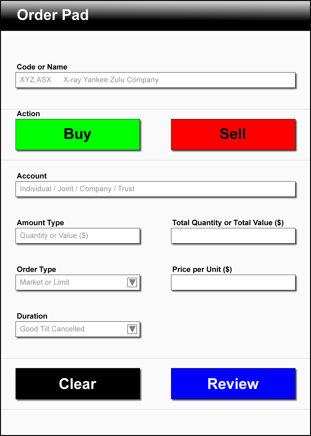
There are primarily two types of orders placed on the market.

  1. Market Orders
  2. Limit Orders


Market Orders

  • Executes at the best available price on the market.
  • Focuses on speed of execution.
  • May convert to a limit order in the event that insufficient quantity exists at market price.


Market to Limit Orders

  • The order starts filling at market price. In the event that there is insufficient quantity available at market price, the order may convert to a limit order and remain in the market until fulfilled at that price.


Limit Orders

  • Executes at the price specified.


Price per Unit ($)

  • Only applicable to limit orders
  • Price you wish to buy or sell each unit.


Duration

  • Good For Day: The order will remain in the market until market closure on the day.
  • Good Till Cancelled: The order will remain in the market until such time as it is cancelled.
  • Good Till Date: The order will remain in the market until market closure of the specified date.