Financial Instruments

5 Jun 0

Index	Category	Function	Description
1	Add-in and Automation	CALL	Calls a procedure in a dynamic link library or code resource.
2	Add-in and Automation	EUROCONVERT	Converts a number to euros, converts a number from euros to a euro member currency, or converts a number from one euro member currency to another by using the euro as an intermediary (triangulation).
3	Add-in and Automation	REGISTER.ID	Returns the register ID of the specified dynamic link library (DLL) or code resource that has been previously registered.
4	Compatibility	BETADIST	Returns the beta cumulative distribution function.
5	Compatibility	BETAINV	Returns the inverse of the cumulative distribution function for a specified beta distribution.
6	Compatibility	BINOMDIST	Returns the individual term binomial distribution probability.
7	Compatibility	CEILING	Rounds a number to the nearest integer or to the nearest multiple of significance.
8	Compatibility	CHIDIST	Returns the one-tailed probability of the chi-squared distribution.
9	Compatibility	CHIINV	Returns the inverse of the one-tailed probability of the chi-squared distribution.
10	Compatibility	CHITEST	Returns the test for independence.
11	Compatibility	CONFIDENCE	Returns the confidence interval for a population mean.
12	Compatibility	COVAR	Returns covariance, the average of the products of paired deviations.
13	Compatibility	CRITBINOM	Returns the smallest value for which the cumulative binomial distribution is less than or equal to a criterion value.
14	Compatibility	EXPONDIST	Returns the exponential distribution.
15	Compatibility	FDIST	Returns the F probability distribution.
16	Compatibility	FINV	Returns the inverse of the F probability distribution.
17	Compatibility	FLOOR	Rounds a number down, toward zero.
18	Compatibility	FTEST	Returns the result of an F-test.
19	Compatibility	GAMMADIST	Returns the gamma distribution.
20	Compatibility	GAMMAINV	Returns the inverse of the gamma cumulative distribution.
21	Compatibility	HYPGEOMDIST	Returns the hypergeometric distribution.
22	Compatibility	LOGINV	Returns the inverse of the lognormal cumulative distribution.
23	Compatibility	LOGNORMDIST	Returns the cumulative lognormal distribution.
24	Compatibility	MODE	Returns the most common value in a data set.
25	Compatibility	NEGBINOMDIST	Returns the negative binomial distribution.
26	Compatibility	NORM.INV	Returns the inverse of the normal cumulative distribution.
27	Compatibility	NORMDIST	Returns the normal cumulative distribution.
28	Compatibility	NORMSDIST	Returns the standard normal cumulative distribution.
29	Compatibility	NORMSINV	Returns the inverse of the standard normal cumulative distribution.
30	Compatibility	PERCENTILE	Returns the k-th percentile of values in a range.
31	Compatibility	PERCENTRANK	Returns the percentage rank of a value in a data set.
32	Compatibility	POISSON	Returns the Poisson distribution.
33	Compatibility	QUARTILE	Returns the quartile of a data set.
34	Compatibility	RANK	Returns the rank of a number in a list of numbers.
35	Compatibility	STDEV	Estimates standard deviation based on a sample.
36	Compatibility	STDEVP	Calculates standard deviation based on the entire population.
37	Compatibility	TDIST	Returns the Student's t-distribution.
38	Compatibility	TINV	Returns the inverse of the Student's t-distribution.
39	Compatibility	TTEST	Returns the probability associated with a Student's t-test.
40	Compatibility	VAR	Estimates variance based on a sample.
41	Compatibility	VARP	Calculates variance based on the entire population.
42	Compatibility	WEIBULL	Calculates variance based on the entire population, including numbers, text, and logical values.
43	Compatibility	ZTEST	Returns the one-tailed probability-value of a z-test.
44	Cube	CUBEKPIMEMBER	Returns a key performance indicator (KPI) name, property, and measure, and displays the name and property in the cell. A KPI is a quantifiable measurement, such as monthly gross profit or quarterly employee turnover, used to monitor an organization's performance.
45	Cube	CUBEMEMBER	Returns a member or tuple in a cube hierarchy. Use to validate that the member or tuple exists in the cube.
46	Cube	CUBEMEMBERPROPERTY	Returns the value of a member property in the cube. Use to validate that a member name exists within the cube and to return the specified property for this member.
47	Cube	CUBERANKEDMEMBER	Returns the nth, or ranked, member in a set. Use to return one or more elements in a set, such as the top sales performer or top 10 students.
48	Cube	CUBESET	Defines a calculated set of members or tuples by sending a set expression to the cube on the server, which creates the set, and then returns that set to Microsoft Office Excel.
49	Cube	CUBESETCOUNT	Returns the number of items in a set.
50	Cube	CUBEVALUE	Returns an aggregated value from a cube.
51	Database	DAVERAGE	Returns the average of selected database entries.
52	Database	DCOUNT	Counts the cells that contain numbers in a database.
53	Database	DCOUNTA	Counts nonblank cells in a database.
54	Database	DGET	Extracts from a database a single record that matches the specified criteria.
55	Database	DMAX	Returns the maximum value from selected database entries.
56	Database	DMIN	Returns the minimum value from selected database entries.
57	Database	DPRODUCT	Multiplies the values in a particular field of records that match the criteria in a database.
58	Database	DSTDEV	Estimates the standard deviation based on a sample of selected database entries.
59	Database	DSTDEVP	Calculates the standard deviation based on the entire population of selected database entries.
60	Database	DSUM	Adds the numbers in the field column of records in the database that match the criteria.
61	Database	DVAR	Estimates variance based on a sample from selected database entries.
62	Database	DVARP	Calculates variance based on the entire population of selected database entries.
63	Date and Time	DATE	Returns the serial number of a particular date.
64	Date and Time	DATEDIF	Calculates the number of days, months, or years between two dates. This function is useful in formulas where you need to calculate an age.
65	Date and Time	DATEVALUE	Converts a date in the form of text to a serial number.
66	Date and Time	DAY	Converts a serial number to a day of the month.
67	Date and Time	DAYS	Returns the number of days between two dates.
68	Date and Time	DAYS360	Calculates the number of days between two dates based on a 360-day year.
69	Date and Time	EDATE	Returns the serial number of the date that is the indicated number of months before or after the start date.
70	Date and Time	EOMONTH	Returns the serial number of the last day of the month before or after a specified number of months.
71	Date and Time	HOUR	Converts a serial number to an hour.
72	Date and Time	ISOWEEKNUM	Returns the number of the ISO week number of the year for a given date.
73	Date and Time	MINUTE	Converts a serial number to a minute.
74	Date and Time	MONTH	Converts a serial number to a month.
75	Date and Time	NETWORKDAYS	Returns the number of whole workdays between two dates.
76	Date and Time	NETWORKDAYS.INTL	Returns the number of whole workdays between two dates using parameters to indicate which and how many days are weekend days.
77	Date and Time	NOW	Returns the serial number of the current date and time.
78	Date and Time	SECOND	Converts a serial number to a second.
79	Date and Time	TIME	Returns the serial number of a particular time.
80	Date and Time	TIMEVALUE	Converts a time in the form of text to a serial number.
81	Date and Time	TODAY	Returns the serial number of today's date.
82	Date and Time	WEEKDAY	Converts a serial number to a day of the week.
83	Date and Time	WEEKNUM	Converts a serial number to a number representing where the week falls numerically with a year.
84	Date and Time	WORKDAY	Returns the serial number of the date before or after a specified number of workdays.
85	Date and Time	WORKDAY.INTL	Returns the serial number of the date before or after a specified number of workdays using parameters to indicate which and how many days are weekend days.
86	Date and Time	YEAR	Converts a serial number to a year.
87	Date and Time	YEARFRAC	Returns the year fraction representing the number of whole days between start_date and end_date.
88	Engineering	BESSELI	Returns the modified Bessel function In(x).
89	Engineering	BESSELJ	Returns the Bessel function Jn(x).
90	Engineering	BESSELK	Returns the modified Bessel function Kn(x).
91	Engineering	BESSELY	Returns the Bessel function Yn(x).
92	Engineering	BIN2DEC	Converts a binary number to decimal.
93	Engineering	BIN2HEX	Converts a binary number to hexadecimal.
94	Engineering	BIN2OCT	Converts a binary number to octal.
95	Engineering	BITAND	Returns a 'Bitwise And' of two numbers.
96	Engineering	BITLSHIFT	Returns a value number shifted left by shift_amount bits.
97	Engineering	BITOR	Returns a bitwise OR of 2 numbers.
98	Engineering	BITRSHIFT	Returns a value number shifted right by shift_amount bits.
99	Engineering	BITXOR	Returns a bitwise 'Exclusive Or' of two numbers.
100	Engineering	COMPLEX	Converts real and imaginary coefficients into a complex number.
101	Engineering	CONVERT	Converts a number from one measurement system to another.
102	Engineering	DEC2BIN	Converts a decimal number to binary.
103	Engineering	DEC2HEX	Converts a decimal number to hexadecimal.
104	Engineering	DEC2OCT	Converts a decimal number to octal.
105	Engineering	DELTA	Tests whether two values are equal.
106	Engineering	ERF	Returns the error function.
107	Engineering	ERF.PRECISE	Returns the error function.
108	Engineering	ERFC	Returns the complementary error function.
109	Engineering	ERFC.PRECISE	Returns the complementary ERF function integrated between x and infinity.
110	Engineering	GESTEP	Tests whether a number is greater than a threshold value.
111	Engineering	HEX2BIN	Converts a hexadecimal number to binary.
112	Engineering	HEX2DEC	Converts a hexadecimal number to decimal.
113	Engineering	HEX2OCT	Converts a hexadecimal number to octal.
114	Engineering	IMABS	Returns the absolute value (modulus) of a complex number.
115	Engineering	IMAGINARY	Returns the imaginary coefficient of a complex number.
116	Engineering	IMARGUMENT	Returns the argument theta, an angle expressed in radians.
117	Engineering	IMCONJUGATE	Returns the complex conjugate of a complex number.
118	Engineering	IMCOS	Returns the cosine of a complex number.
119	Engineering	IMCOSH	Returns the hyperbolic cosine of a complex number.
120	Engineering	IMCOT	Returns the cotangent of a complex number.
121	Engineering	IMCSC	Returns the cosecant of a complex number.
122	Engineering	IMCSCH	Returns the hyperbolic cosecant of a complex number.
123	Engineering	IMDIV	Returns the quotient of two complex numbers.
124	Engineering	IMEXP	Returns the exponential of a complex number.
125	Engineering	IMLN	Returns the natural logarithm of a complex number.
126	Engineering	IMLOG10	Returns the base-10 logarithm of a complex number.
127	Engineering	IMLOG2	Returns the base-2 logarithm of a complex number.
128	Engineering	IMPOWER	Returns a complex number raised to an integer power.
129	Engineering	IMPRODUCT	Returns the product of complex numbers.
130	Engineering	IMREAL	Returns the real coefficient of a complex number.
131	Engineering	IMSEC	Returns the secant of a complex number.
132	Engineering	IMSECH	Returns the hyperbolic secant of a complex number.
133	Engineering	IMSIN	Returns the sine of a complex number.
134	Engineering	IMSINH	Returns the hyperbolic sine of a complex number.
135	Engineering	IMSQRT	Returns the square root of a complex number.
136	Engineering	IMSUB	Returns the difference between two complex numbers.
137	Engineering	IMSUM	Returns the sum of complex numbers.
138	Engineering	IMTAN	Returns the tangent of a complex number.
139	Engineering	OCT2BIN	Converts an octal number to binary.
140	Engineering	OCT2DEC	Converts an octal number to decimal.
141	Engineering	OCT2HEX	Converts an octal number to hexadecimal.
142	Financial	ACCRINT	Returns the accrued interest for a security that pays periodic interest.
143	Financial	ACCRINTM	Returns the accrued interest for a security that pays interest at maturity.
144	Financial	AMORDEGRC	Returns the depreciation for each accounting period by using a depreciation coefficient.
145	Financial	AMORLINC	Returns the depreciation for each accounting period.
146	Financial	COUPDAYBS	Returns the number of days from the beginning of the coupon period to the settlement date.
147	Financial	COUPDAYS	Returns the number of days in the coupon period that contains the settlement date.
148	Financial	COUPDAYSNC	Returns the number of days from the settlement date to the next coupon date.
149	Financial	COUPNCD	Returns the next coupon date after the settlement date.
150	Financial	COUPNUM	Returns the number of coupons payable between the settlement date and maturity date.
151	Financial	COUPPCD	Returns the previous coupon date before the settlement date.
152	Financial	CUMIPMT	Returns the cumulative interest paid between two periods.
153	Financial	CUMPRINC	Returns the cumulative principal paid on a loan between two periods.
154	Financial	DB	Returns the depreciation of an asset for a specified period by using the fixed-declining balance method.
155	Financial	DDB	Returns the depreciation of an asset for a specified period by using the double-declining balance method or some other method that you specify.
156	Financial	DISC	Returns the discount rate for a security.
157	Financial	DOLLARDE	Converts a dollar price, expressed as a fraction, into a dollar price, expressed as a decimal number.
158	Financial	DOLLARFR	Converts a dollar price, expressed as a decimal number, into a dollar price, expressed as a fraction.
159	Financial	DURATION	Returns the annual duration of a security with periodic interest payments.
160	Financial	EFFECT	Returns the effective annual interest rate.
161	Financial	FV	Returns the future value of an investment.
162	Financial	FVSCHEDULE	Returns the future value of an initial principal after applying a series of compound interest rates.
163	Financial	INTRATE	Returns the interest rate for a fully invested security.
164	Financial	IPMT	Returns the interest payment for an investment for a given period.
165	Financial	IRR	Returns the internal rate of return for a series of cash flows.
166	Financial	ISPMT	Calculates the interest paid during a specific period of an investment.
167	Financial	MDURATION	Returns the Macauley modified duration for a security with an assumed par value of $100.
168	Financial	MIRR	Returns the internal rate of return where positive and negative cash flows are financed at different rates.
169	Financial	NOMINAL	Returns the annual nominal interest rate.
170	Financial	NPER	Returns the number of periods for an investment.
171	Financial	NPV	Returns the net present value of an investment based on a series of periodic cash flows and a discount rate.
172	Financial	ODDFPRICE	Returns the price per $100 face value of a security with an odd first period.
173	Financial	ODDFYIELD	Returns the yield of a security with an odd first period.
174	Financial	ODDLPRICE	Returns the price per $100 face value of a security with an odd last period.
175	Financial	ODDLYIELD	Returns the yield of a security with an odd last period.
176	Financial	PDURATION	Returns the number of periods required by an investment to reach a specified value.
177	Financial	PMT	Returns the periodic payment for an annuity.
178	Financial	PPMT	Returns the payment on the principal for an investment for a given period.
179	Financial	PRICE	Returns the price per $100 face value of a security that pays periodic interest.
180	Financial	PRICEDISC	Returns the price per $100 face value of a discounted security.
181	Financial	PRICEMAT	Returns the price per $100 face value of a security that pays interest at maturity.
182	Financial	PV	Returns the present value of an investment.
183	Financial	RATE	Returns the interest rate per period of an annuity.
184	Financial	RECEIVED	Returns the amount received at maturity for a fully invested security.
185	Financial	RRI	Returns an equivalent interest rate for the growth of an investment.
186	Financial	SLN	Returns the straight-line depreciation of an asset for one period.
187	Financial	SYD	Returns the sum-of-years' digits depreciation of an asset for a specified period.
188	Financial	TBILLEQ	Returns the bond-equivalent yield for a Treasury bill.
189	Financial	TBILLPRICE	Returns the price per $100 face value for a Treasury bill.
190	Financial	TBILLYIELD	Returns the yield for a Treasury bill.
191	Financial	VDB	Returns the depreciation of an asset for a specified or partial period by using a declining balance method.
192	Financial	XIRR	Returns the internal rate of return for a schedule of cash flows that is not necessarily periodic.
193	Financial	XNPV	Returns the net present value for a schedule of cash flows that is not necessarily periodic.
194	Financial	YIELD	Returns the yield on a security that pays periodic interest.
195	Financial	YIELDDISC	Returns the annual yield for a discounted security; for example, a Treasury bill.
196	Financial	YIELDMAT	Returns the annual yield of a security that pays interest at maturity.
197	Information	CELL	Returns information about the formatting, location, or contents of a cell.
198	Information	ERROR.TYPE	Returns a number corresponding to an error type.
199	Information	INFO	Returns information about the current operating environment.
200	Information	ISBLANK	Returns TRUE if the value is blank.
201	Information	ISERR	Returns TRUE if the value is any error value except #N/A.
202	Information	ISERROR	Returns TRUE if the value is any error value.
203	Information	ISEVEN	Returns TRUE if the number is even.
204	Information	ISFORMULA	Returns TRUE if there is a reference to a cell that contains a formula.
205	Information	ISLOGICAL	Returns TRUE if the value is a logical value.
206	Information	ISNA	Returns TRUE if the value is the #N/A error value.
207	Information	ISNONTEXT	Returns TRUE if the value is not text.
208	Information	ISNUMBER	Returns TRUE if the value is a number.
209	Information	ISODD	Returns TRUE if the number is odd.
210	Information	ISOMITTED	Checks whether the value in a LAMBDA is missing and returns TRUE or FALSE.
211	Information	ISREF	Returns TRUE if the value is a reference.
212	Information	ISTEXT	Returns TRUE if the value is text.
213	Information	N	Returns a value converted to a number.
214	Information	NA	Returns the error value #N/A.
215	Information	SHEET	Returns the sheet number of the referenced sheet.
216	Information	SHEETS	Returns the number of sheets in a reference.
217	Information	STOCKHISTORY	Retrieves historical data about a financial instrument.
218	Information	STOCKHISTORY	Retrieves historical data about a financial instrument and loads it as an array.
219	Information	TYPE	Returns a number indicating the data type of a value.
220	Logical	AND	Returns TRUE if all of its arguments are TRUE.
221	Logical	BYCOL	Applies a LAMBDA to each column and returns an array of the results.
222	Logical	BYROW	Applies a LAMBDA to each row and returns an array of the results.
223	Logical	IF	Specifies a logical test to perform.
224	Logical	IFERROR	Returns a value you specify if a formula evaluates to an error; otherwise, returns the result of the formula.
225	Logical	IFNA	Returns the value you specify if the expression resolves to #N/A, otherwise returns the result of the expression.
226	Logical	IFS	Checks whether one or more conditions are met and returns a value that corresponds to the first TRUE condition.
227	Logical	LAMBDA	Create custom, reusable and call them by a friendly name.
228	Logical	LET	Assigns names to calculation results.
229	Logical	MAKEARRAY	Returns a calculated array of a specified row and column size, by applying a LAMBDA.
230	Logical	MAP	Returns an array formed by mapping each value in the array(s) to a new value by applying a LAMBDA to create a new value.
231	Logical	NOT	Reverses the logic of its argument.
232	Logical	OR	Returns TRUE if any argument is TRUE.
233	Logical	REDUCE	Reduces an array to an accumulated value by applying a LAMBDA to each value and returning the total value in the accumulator.
234	Logical	SCAN	Scans an array by applying a LAMBDA to each value and returns an array that has each intermediate value.
235	Logical	SWITCH	Evaluates an expression against a list of values and returns the result corresponding to the first matching value. If there is no match, an optional default value may be returned.
236	Logical	XOR	Returns a logical exclusive OR of all arguments.
237	Logical		Returns the logical value FALSE.
238	Logical	1	Returns the logical value TRUE.
239	Look and Reference	VSTACK	Appends arrays vertically and in sequence to return a larger array.
240	Look and Reference	WRAPCOLS	Wraps the provided row or column of values by columns after a specified number of elements.
241	Look and Reference	WRAPROWS	Wraps the provided row or column of values by rows after a specified number of elements.
242	Lookup and Reference	ADDRESS	Returns a reference as text to a single cell in a worksheet.
243	Lookup and Reference	AREAS	Returns the number of areas in a reference.
244	Lookup and Reference	CHOOSE	Chooses a value from a list of values.
245	Lookup and Reference	CHOOSECOLS	Returns the specified columns from an array.
246	Lookup and Reference	CHOOSEROWS	Returns the specified rows from an array.
247	Lookup and Reference	COLUMN	Returns the column number of a reference.
248	Lookup and Reference	COLUMNS	Returns the number of columns in a reference.
249	Lookup and Reference	DROP	Excludes a specified number of rows or columns from the start or end of an array.
250	Lookup and Reference	EXPAND	Expands or pads an array to specified row and column dimensions.
251	Lookup and Reference	FILTER	Filters a range of data based on criteria you define.
252	Lookup and Reference	FORMULATEXT	Returns the formula at the given reference as text.
253	Lookup and Reference	GETPIVOTDATA	Returns data stored in a PivotTable report.
254	Lookup and Reference	GROUPBY	Helps a user group, aggregate, sort, and filter data based on the fields you specify.
255	Lookup and Reference	HLOOKUP	Looks in the top row of an array and returns the value of the indicated cell.
256	Lookup and Reference	HSTACK	Appends arrays horizontally and in sequence to return a larger array.
257	Lookup and Reference	HYPERLINK	Creates a shortcut or jump that opens a document stored on a network server, an intranet, or the Internet.
258	Lookup and Reference	IMAGE	urns an image from a given source.
259	Lookup and Reference	INDEX	Uses an index to choose a value from a reference or array.
260	Lookup and Reference	INDIRECT	Returns a reference indicated by a text value.
261	Lookup and Reference	LOOKUP	Looks up values in a vector or array.
262	Lookup and Reference	MATCH	Looks up values in a reference or array.
263	Lookup and Reference	OFFSET	Returns a reference offset from a given reference.
264	Lookup and Reference	PIVOTBY	Helps a user group, aggregate, sort, and filter data based on the row and column fields that you specify.
265	Lookup and Reference	ROW	Returns the row number of a reference.
266	Lookup and Reference	ROWS	Returns the number of rows in a reference.
267	Lookup and Reference	RTD	Retrieves real-time data from a program that supports COM automation.
268	Lookup and Reference	SORT	Sorts the contents of a range or array.
269	Lookup and Reference	SORTBY	Sorts the contents of a range or array based on the values in a corresponding range or array.
270	Lookup and Reference	TAKE	Returns a specified number of contiguous rows or columns from the start or end of an array.
271	Lookup and Reference	TOCOL	Returns the array in a single column.
272	Lookup and Reference	TOROW	Returns the array in a single row.
273	Lookup and Reference	TRANSPOSE	Returns the transpose of an array.
274	Lookup and Reference	TRIMRANGE	Scans in from the edges of a range or array until it finds a non-blank cell (or value), it then excludes those blank rows or columns.
275	Lookup and Reference	UNIQUE	Returns a list of unique values in a list or range.
276	Lookup and Reference	VLOOKUP	Looks in the first column of an array and moves across the row to return the value of a cell.
277	Lookup and Reference	XLOOKUP	Searches a range or an array, and returns an item corresponding to the first match it finds. If a match doesn't exist, then XLOOKUP can return the closest (approximate) match.
278	Lookup and Reference	XMATCH	Returns the relative position of an item in an array or range of cells. .
279	Math and Trigonometry	ABS	Returns the absolute value of a number.
280	Math and Trigonometry	ACOS	Returns the arccosine of a number.
281	Math and Trigonometry	ACOSH	Returns the inverse hyperbolic cosine of a number.
282	Math and Trigonometry	ACOT	Returns the arccotangent of a number.
283	Math and Trigonometry	ACOTH	Returns the hyperbolic arccotangent of a number.
284	Math and Trigonometry	AGGREGATE	Returns an aggregate in a list or database.
285	Math and Trigonometry	ARABIC	Converts a Roman number to Arabic, as a number.
286	Math and Trigonometry	ASIN	Returns the arcsine of a number.
287	Math and Trigonometry	ASINH	Returns the inverse hyperbolic sine of a number.
288	Math and Trigonometry	ATAN	Returns the arctangent of a number.
289	Math and Trigonometry	ATAN2	Returns the arctangent from x- and y-coordinates.
290	Math and Trigonometry	ATANH	Returns the inverse hyperbolic tangent of a number.
291	Math and Trigonometry	BASE	Converts a number into a text representation with the given radix (base).
292	Math and Trigonometry	CEILING.MATH	Rounds a number up, to the nearest integer or to the nearest multiple of significance.
293	Math and Trigonometry	CEILING.PRECISE	Rounds a number the nearest integer or to the nearest multiple of significance. Regardless of the sign of the number, the number is rounded up.
294	Math and Trigonometry	COMBIN	Returns the number of combinations for a given number of objects.
295	Math and Trigonometry	COMBINA	.
296	Math and Trigonometry	COS	Returns the cosine of a number.
297	Math and Trigonometry	COSH	Returns the hyperbolic cosine of a number.
298	Math and Trigonometry	COT	Returns the hyperbolic cosine of a number.
299	Math and Trigonometry	COTH	Returns the cotangent of an angle.
300	Math and Trigonometry	CSC	Returns the cosecant of an angle.
301	Math and Trigonometry	CSCH	Returns the hyperbolic cosecant of an angle.
302	Math and Trigonometry	DECIMAL	Converts a text representation of a number in a given base into a decimal number.
303	Math and Trigonometry	DEGREES	Converts radians to degrees.
304	Math and Trigonometry	EVEN	Rounds a number up to the nearest even integer.
305	Math and Trigonometry	EXP	Returns e raised to the power of a given number.
306	Math and Trigonometry	FACT	Returns the factorial of a number.
307	Math and Trigonometry	FACTDOUBLE	Returns the double factorial of a number.
308	Math and Trigonometry	FLOOR.MATH	Rounds a number down, to the nearest integer or to the nearest multiple of significance.
309	Math and Trigonometry	FLOOR.PRECISE	Rounds a number the nearest integer or to the nearest multiple of significance. Regardless of the sign of the number, the number is rounded up.
310	Math and Trigonometry	GCD	Returns the greatest common divisor.
311	Math and Trigonometry	INT	Rounds a number down to the nearest integer.
312	Math and Trigonometry	ISO.CEILING	Returns a number that is rounded up to the nearest integer or to the nearest multiple of significance.
313	Math and Trigonometry	LCM	Returns the least common multiple.
314	Math and Trigonometry	LN	Returns the natural logarithm of a number.
315	Math and Trigonometry	LOG	Returns the logarithm of a number to a specified base.
316	Math and Trigonometry	LOG10	Returns the base-10 logarithm of a number.
317	Math and Trigonometry	MDETERM	Returns the matrix determinant of an array.
318	Math and Trigonometry	MINVERSE	Returns the matrix inverse of an array.
319	Math and Trigonometry	MMULT	Returns the matrix product of two arrays.
320	Math and Trigonometry	MOD	Returns the remainder from division.
321	Math and Trigonometry	MROUND	Returns a number rounded to the desired multiple.
322	Math and Trigonometry	MULTINOMIAL	Returns the multinomial of a set of numbers.
323	Math and Trigonometry	MUNIT	Returns the unit matrix or the specified dimension.
324	Math and Trigonometry	ODD	Rounds a number up to the nearest odd integer.
325	Math and Trigonometry	PERCENTOF	Sums the values in the subset and divides it by all the values.
326	Math and Trigonometry	PI	Returns the value of pi.
327	Math and Trigonometry	POWER	Returns the result of a number raised to a power.
328	Math and Trigonometry	PRODUCT	Multiplies its arguments.
329	Math and Trigonometry	QUOTIENT	Returns the integer portion of a division.
330	Math and Trigonometry	RADIANS	Converts degrees to radians.
331	Math and Trigonometry	RAND	Returns a random number between 0 and 1.
332	Math and Trigonometry	RANDARRAY	Returns an array of random numbers between 0 and 1. However, you can specify the number of rows and columns to fill, minimum and maximum values, and whether to return whole numbers or decimal values.
333	Math and Trigonometry	RANDBETWEEN	Returns a random number between the numbers you specify.
334	Math and Trigonometry	ROMAN	Converts an arabic numeral to roman, as text.
335	Math and Trigonometry	ROUND	Rounds a number to a specified number of digits.
336	Math and Trigonometry	ROUNDDOWN	Rounds a number down, toward zero.
337	Math and Trigonometry	ROUNDUP	Rounds a number up, away from zero.
338	Math and Trigonometry	SEC	Returns the secant of an angle.
339	Math and Trigonometry	SECH	Returns the hyperbolic secant of an angle.
340	Math and Trigonometry	SEQUENCE	Generates a list of sequential numbers in an array, such as 1, 2, 3, 4.
341	Math and Trigonometry	SERIESSUM	Returns the sum of a power series based on the formula.
342	Math and Trigonometry	SIGN	Returns the sign of a number.
343	Math and Trigonometry	SIN	Returns the sine of the given angle.
344	Math and Trigonometry	SINH	Returns the hyperbolic sine of a number.
345	Math and Trigonometry	SQRT	Returns a positive square root.
346	Math and Trigonometry	SQRTPI	Returns the square root of (number * pi).
347	Math and Trigonometry	SUBTOTAL	Returns a subtotal in a list or database.
348	Math and Trigonometry	SUM	Adds its arguments.
349	Math and Trigonometry	SUMIF	Adds the cells specified by a given criteria.
350	Math and Trigonometry	SUMIFS	Adds the cells in a range that meet multiple criteria.
351	Math and Trigonometry	SUMPRODUCT	Returns the sum of the products of corresponding array components.
352	Math and Trigonometry	SUMSQ	Returns the sum of the squares of the arguments.
353	Math and Trigonometry	SUMX2MY2	Returns the sum of the difference of squares of corresponding values in two arrays.
354	Math and Trigonometry	SUMX2PY2	Returns the sum of the sum of squares of corresponding values in two arrays.
355	Math and Trigonometry	SUMXMY2	Returns the sum of squares of differences of corresponding values in two arrays.
356	Math and Trigonometry	TAN	Returns the tangent of a number.
357	Math and Trigonometry	TANH	Returns the hyperbolic tangent of a number.
358	Math and Trigonometry	TRUNC	Truncates a number to an integer.
359	Returns the number of		Returns the number of combinations with repetitions for a given number of items.
360	Statistical	AVEDEV	Returns the average of the absolute deviations of data points from their mean.
361	Statistical	AVERAGE	Returns the average of its arguments.
362	Statistical	AVERAGEA	Returns the average of its arguments, including numbers, text, and logical values.
363	Statistical	AVERAGEIF	Returns the average (arithmetic mean) of all the cells in a range that meet a given criteria.
364	Statistical	AVERAGEIFS	Returns the average (arithmetic mean) of all cells that meet multiple criteria.
365	Statistical	BETA.DIST	Returns the beta cumulative distribution function.
366	Statistical	BETA.INVn	Returns the inverse of the cumulative distribution function for a specified beta distribution.
367	Statistical	BINOM.DIST	Returns the individual term binomial distribution probability.
368	Statistical	BINOM.DIST.RANGE	Returns the probability of a trial result using a binomial distribution.
369	Statistical	BINOM.INV	Returns the smallest value for which the cumulative binomial distribution is less than or equal to a criterion value.
370	Statistical	CHISQ.DIST	Returns the cumulative beta probability density function.
371	Statistical	CHISQ.DIST.RT	Returns the one-tailed probability of the chi-squared distribution.
372	Statistical	CHISQ.INV	Returns the cumulative beta probability density function.
373	Statistical	CHISQ.INV.RT	Returns the inverse of the one-tailed probability of the chi-squared distribution.
374	Statistical	CHISQ.TEST	Returns the test for independence.
375	Statistical	CONFIDENCE.NORM	Returns the confidence interval for a population mean.
376	Statistical	CONFIDENCE.T	Returns the confidence interval for a population mean, using a Student's t distribution.
377	Statistical	CORREL	Returns the correlation coefficient between two data sets.
378	Statistical	COUNT	Counts how many numbers are in the list of arguments.
379	Statistical	COUNTA	Counts how many values are in the list of arguments.
380	Statistical	COUNTBLANK	Counts the number of blank cells within a range.
381	Statistical	COUNTIF	Counts the number of cells within a range that meet the given criteria.
382	Statistical	COUNTIFS	Counts the number of cells within a range that meet multiple criteria.
383	Statistical	COVARIANCE.P	Returns covariance, the average of the products of paired deviations.
384	Statistical	COVARIANCE.S	Returns the sample covariance, the average of the products deviations for each data point pair in two data sets.
385	Statistical	DEVSQ	Returns the sum of squares of deviations.
386	Statistical	EXPON.DIST	Returns the exponential distribution.
387	Statistical	F.DIST	Returns the F probability distribution.
388	Statistical	F.DIST.RT	Returns the F probability distribution.
389	Statistical	F.INV	Returns the inverse of the F probability distribution.
390	Statistical	F.INV.RT	Returns the inverse of the F probability distribution.
391	Statistical	F.TEST	Returns the result of an F-test.
392	Statistical	FISHER	Returns the Fisher transformation.
393	Statistical	FISHERINV	Returns the inverse of the Fisher transformation.
394	Statistical	FORECAST	Returns a value along a linear trend.
395	Statistical	FORECAST.ETS	Returns a future value based on existing (historical) values by using the AAA version of the Exponential Smoothing (ETS) algorithm.
396	Statistical	FORECAST.ETS.CONFINT	Returns a confidence interval for the forecast value at the specified target date.
397	Statistical	FORECAST.ETS.SEASONALITY	Returns the length of the repetitive pattern Excel detects for the specified time series.
398	Statistical	FORECAST.ETS.STAT	Returns a statistical value as a result of time series forecasting.
399	Statistical	FORECAST.LINEAR	Returns a future value based on existing values.
400	Statistical	FREQUENCY	Returns a frequency distribution as a vertical array.
401	Statistical	GAMMA	Returns the Gamma function value.
402	Statistical	GAMMA.DIST	Returns the gamma distribution.
403	Statistical	GAMMA.INV	Returns the inverse of the gamma cumulative distribution.
404	Statistical	GAMMALN	Returns the natural logarithm of the gamma function, Γ(x).
405	Statistical	GAMMALN.PRECISE	Returns the natural logarithm of the gamma function, Γ(x).
406	Statistical	GAUSS	Returns 0.5 less than the standard normal cumulative distribution.
407	Statistical	GEOMEAN	Returns the geometric mean.
408	Statistical	GROWTH	Returns values along an exponential trend.
409	Statistical	HARMEAN	Returns the harmonic mean.
410	Statistical	HYPGEOM.DIST	Returns the hypergeometric distribution.
411	Statistical	INTERCEPT	Returns the intercept of the linear regression line.
412	Statistical	KURT	Returns the kurtosis of a data set.
413	Statistical	LARGE	Returns the k-th largest value in a data set.
414	Statistical	LINEST	Returns the parameters of a linear trend.
415	Statistical	LOGEST	Returns the parameters of an exponential trend.
416	Statistical	LOGNORM.DIST	Returns the cumulative lognormal distribution.
417	Statistical	LOGNORM.INV	Returns the inverse of the lognormal cumulative distribution.
418	Statistical	MAX	Returns the maximum value in a list of arguments.
419	Statistical	MAXA	Returns the maximum value in a list of arguments, including numbers, text, and logical values.
420	Statistical	MAXIFS	Returns the maximum value among cells specified by a given set of conditions or criteria.
421	Statistical	MEDIAN	Returns the median of the given numbers.
422	Statistical	MIN	Returns the minimum value in a list of arguments.
423	Statistical	MINA	Returns the smallest value in a list of arguments, including numbers, text, and logical values.
424	Statistical	MINIFS	Returns the minimum value among cells specified by a given set of conditions or criteria.
425	Statistical	MODE.MULT	Returns a vertical array of the most frequently occurring, or repetitive values in an array or range of data.
426	Statistical	MODE.SNGL	Returns the most common value in a data set.
427	Statistical	NEGBINOM.DIST	Returns the negative binomial distribution.
428	Statistical	NORM.DIST	Returns the normal cumulative distribution.
429	Statistical	NORM.S.DIST	Returns the standard normal cumulative distribution.
430	Statistical	NORM.S.INV	Returns the inverse of the standard normal cumulative distribution.
431	Statistical	NORMINV	Returns the inverse of the normal cumulative distribution.
432	Statistical	PEARSON	Returns the Pearson product moment correlation coefficient.
433	Statistical	PERCENTILE.EXC	Returns the k-th percentile of values in a range, where k is in the range 0.1, exclusive.
434	Statistical	PERCENTILE.INC	Returns the k-th percentile of values in a range.
435	Statistical	PERCENTRANK.EXC	Returns the rank of a value in a data set as a percentage (0.1, exclusive) of the data set.
436	Statistical	PERCENTRANK.INC	Returns the percentage rank of a value in a data set.
437	Statistical	PERMUT	Returns the number of permutations for a given number of objects.
438	Statistical	PERMUTATIONA	Returns the number of permutations for a given number of objects (with repetitions) that can be selected from the total objects.
439	Statistical	PHI	Returns the value of the density function for a standard normal distribution.
440	Statistical	POISSON.DIST	Returns the Poisson distribution.
441	Statistical	PROB	Returns the probability that values in a range are between two limits.
442	Statistical	QUARTILE.EXC	Returns the quartile of the data set, based on percentile values from 0.1, exclusive.
443	Statistical	QUARTILE.INC	Returns the quartile of a data set.
444	Statistical	RANK.AVG	Returns the rank of a number in a list of numbers.
445	Statistical	RANK.EQ	Returns the rank of a number in a list of numbers.
446	Statistical	RSQ	Returns the square of the Pearson product moment correlation coefficient.
447	Statistical	SKEW	Returns the skewness of a distribution.
448	Statistical	SKEW.P	Returns the skewness of a distribution based on a population a characterization of the degree of asymmetry of a distribution around its mean.
449	Statistical	SLOPE	Returns the slope of the linear regression line.
450	Statistical	SMALL	Returns the k-th smallest value in a data set.
451	Statistical	STANDARDIZE	Returns a normalized value.
452	Statistical	STDEV.P	Calculates standard deviation based on the entire population.
453	Statistical	STDEV.S	Estimates standard deviation based on a sample.
454	Statistical	STDEVA	Estimates standard deviation based on a sample, including numbers, text, and logical values.
455	Statistical	STDEVPA	Calculates standard deviation based on the entire population, including numbers, text, and logical values.
456	Statistical	STEYX	Returns the standard error of the predicted y-value for each x in the regression.
457	Statistical	T.DIST	Returns the Percentage Points (probability) for the Student t-distribution.
458	Statistical	T.DIST.2T	Returns the Percentage Points (probability) for the Student t-distribution.
459	Statistical	T.DIST.RT	Returns the Student's t-distribution.
460	Statistical	T.INV	Returns the t-value of the Student's t-distribution as a function of the probability and the degrees of freedom.
461	Statistical	T.INV.2T	Returns the inverse of the Student's t-distribution.
462	Statistical	T.TEST	Returns the probability associated with a Student's t-test.
463	Statistical	TREND	Returns values along a linear trend.
464	Statistical	TRIMMEAN	Returns the mean of the interior of a data set.
465	Statistical	VAR.P	Calculates variance based on the entire population.
466	Statistical	VAR.S	Estimates variance based on a sample.
467	Statistical	VARA	Estimates variance based on a sample, including numbers, text, and logical values.
468	Statistical	VARPA	Calculates variance based on the entire population, including numbers, text, and logical values.
469	Statistical	WEIBULL.DIST	Returns the Weibull distribution.
470	Statistical	Z.TEST	Returns the one-tailed probability-value of a z-test.
471	Text	ARRAYTOTEXT	Returns an array of text values from any specified range.
472	Text	ASC	Changes full-width (double-byte) English letters or katakana within a character string to half-width (single-byte) characters.
473	Text	BAHTTEXT	Converts a number to text, using the ß (baht) currency format.
474	Text	CHAR	Returns the character specified by the code number.
475	Text	CLEAN	Removes all nonprintable characters from text.
476	Text	CODE	Returns a numeric code for the first character in a text string.
477	Text	CONCAT	Combines the text from multiple ranges and/or strings, but it doesn't provide the delimiter or IgnoreEmpty arguments.
478	Text	CONCATENATE	Joins several text items into one text item.
479	Text	DBCS	Changes half-width (single-byte) English letters or katakana within a character string to full-width (double-byte) characters.
480	Text	DETECTLANGUAGE	Identifies the language of a specified text.
481	Text	DOLLAR	Converts a number to text, using the $ (dollar) currency format.
482	Text	EXACT	Checks to see if two text values are identical.
483	Text	FIND, FINDB	Finds one text value within another (case-sensitive).
484	Text	FIXED	Formats a number as text with a fixed number of decimals.
485	Text	JIS	Changes half-width (single-byte) characters within a string to full-width (double-byte) characters.
486	Text	LEFT, LEFTB	Returns the leftmost characters from a text value.
487	Text	LEN, LENB	Returns the number of characters in a text string.
488	Text	LOWER	Converts text to lowercase.
489	Text	MID, MIDB	Returns a specific number of characters from a text string starting at the position you specify.
490	Text	NUMBERVALUE	Converts text to number in a locale-independent manner.
491	Text	PHONETIC	Extracts the phonetic (furigana) characters from a text string.
492	Text	PROPER	Capitalizes the first letter in each word of a text value.
493	Text	REGEXEXTRACT	Extracts strings within the provided text that matches the pattern.
494	Text	REGEXREPLACE	Replaces strings within the provided text that matches the pattern with replacement.
495	Text	REGEXTEST	Determines whether any part of text matches the pattern.
496	Text	REPLACE, REPLACEB	Replaces characters within text.
497	Text	REPT	Repeats text a given number of times.
498	Text	RIGHT, RIGHTB	Returns the rightmost characters from a text value.
499	Text	SEARCH, SEARCHB	Finds one text value within another (not case-sensitive).
500	Text	SUBSTITUTE	Substitutes new text for old text in a text string.

Protected: Fixed Income (Debt) Securities

Admin

Financial Analysis, Financial Instruments

27 Jan 0

Uppercase	Lowercase	Name
Α	α	alpha
Β	β	beta
Γ	γ	gamma
Δ	δ	delta
Ε	ε	epsilon
Ζ	ζ	zêta
Η	η	êta
Θ	θ	thêta
Ι	ι	iota
Κ	κ	kappa
Λ	λ	lambda
Μ	μ	mu
Ν	ν	nu
Ξ	ξ	xi
Ο	ο	omikron
Π	π	pi
Ρ	ρ	rho
Σ	σ, ς	sigma
Τ	τ	tau
Υ	υ	upsilon
Φ	φ	phi
Χ	χ	chi
Ψ	ψ	psi
Ω	ω	omega

Parameter	Description
S₀	spot price at inception of the contract (t=0)
FP	forward price
R_f	annual risk-free rate
T	forward contract term (years)

Mark-to-market is an accounting practice or process that involves adjusting the value of an asset or a liability to reflect its current market value rather than its book value or historical cost. The goal of MTM is to ensure that financial statements reflect the true current value of assets and liabilities as determined by the latest market prices.

In the context of futures contracts, MTM refers to the daily process of revaluing the contract based on the market’s closing price and adjusting the margin accounts of the involved parties accordingly.

The MTM Process in Futures Contracts

Daily Revaluation:
- Futures contracts are marked-to-market at the end of each trading day based on the closing price of the underlying asset. This means that the contract is revalued to reflect the most up-to-date market conditions, essentially recalculating what the contract is worth at that moment.
- The contract’s price moves according to the underlying asset’s price fluctuations. If the futures price rises or falls relative to the previous day’s settlement price, the value of the futures contract will change.
Settlement of Gains and Losses:
- The difference between the closing price of the futures contract at the end of each day and the price at the previous day’s close represents the gain or loss.
- If the value of the futures contract increases (for the holder of a long position, or a “buyer”), the buyer gains, and the seller loses by the same amount. If the value decreases, the seller gains, and the buyer loses by the same amount.
- These gains and losses are settled daily, meaning that they are either credited or debited to the margin accounts of the traders. This daily settlement process prevents the accumulation of large losses over time.
Margin Requirements:
- Initial Margin: This is the amount of money a trader must deposit with the exchange to open a position. It’s a good faith deposit to ensure the trader can fulfill their financial obligations in the contract.
- Maintenance Margin: This is the minimum balance required in a trader’s margin account to keep a position open. If the balance in the margin account drops below this level due to daily losses, the trader receives a margin call and must deposit additional funds to bring the margin back up to the required level.
- The initial margin is the amount needed to enter the position, while the maintenance margin is the threshold below which the position will be liquidated if additional funds are not added.
Resetting the Contract’s Value to Zero:
- The contract’s value is reset to zero at the end of each trading day after gains and losses are settled. This means that traders are not holding on to the profit or loss from the previous day but instead, are working with a fresh starting point for the next day.

Key Features of Mark-to-Market

Real-Time Reflection of Market Conditions: MTM ensures that the value of the futures contract is always aligned with the current market value of the underlying asset. This helps to maintain transparency and accuracy in financial reporting, as the value is updated to reflect what the asset is worth at any given moment.
Reduces Counterparty Risk: By adjusting the value of contracts daily and settling gains and losses regularly, MTM helps reduce the risk that a counterparty may default on their obligations. The daily settlements mean that traders are always on top of their positions, and their exposure is not allowed to build up over time.
Liquidity and Flexibility: The daily settlement of gains and losses also helps keep the futures market liquid and dynamic. Traders can quickly adjust their positions, either adding more margin to cover losses or liquidating their position if the market moves unfavorably.

Why is Mark-to-Market Important?

Transparency and Accuracy: MTM allows for a more accurate reflection of a contract’s value, ensuring that financial statements reflect the true economic value of assets and liabilities.
Regulatory Compliance: Many financial markets and regulatory bodies require the use of MTM accounting to ensure fairness and to minimize systemic risk, particularly in markets like futures and other derivative contracts.
Risk Management: MTM helps manage and limit risk by ensuring that gains and losses are realized and settled daily, allowing traders to take immediate action if necessary, such as depositing additional margin or closing positions.

Mark-to-Market Outside of Futures Contracts

Mark-to-market is not limited to futures markets—it also applies to a range of other financial assets, including:

Equities: Stocks can be marked-to-market at the end of each trading day, adjusting their value to reflect the current market price.
Bonds: Bond prices can be marked-to-market by considering the yield and price of similar instruments in the market.
Derivatives: Options, swaps, and other derivatives are also subject to MTM, which reflects their real-time market value, based on the underlying asset’s current price.

Example of MTM in Action (Futures Contract)

Let’s say a trader enters into a long futures contract on oil with a price of USD 70 per barrel. Here’s how MTM would work:

On Day 1, the futures price is USD 70. The trader deposits an initial margin of USD 5,000.
On Day 2, the price rises to USD 72 per barrel. The trader’s account is credited with the gain of USD 2 per barrel.
On Day 3, the price falls to USD 71. The trader’s account is debited USD 1 per barrel.
On Day 4, the price rises again to USD 73. The trader’s account is credited USD 2 per barrel.

Each day, the trader’s margin account is adjusted according to the daily change in the contract’s value, ensuring that the position is fully collateralized and reflecting the real-time market value of the contract.

Conclusion

Mark-to-market is an essential process for ensuring that the values of financial contracts, particularly in futures markets, are accurately and transparently reflected based on current market conditions. It helps to manage risk, ensure liquidity, and provide up-to-date financial reporting, all while preventing large-scale losses or defaults. The MTM system of daily settlement and revaluation promotes efficiency and stability in financial markets.

Admin

Financial Instruments

22 Jan 0

Risk Premium

A risk premium is the additional return or yield that an investor requires for taking on the extra risk associated with an investment compared to a risk-free alternative. In other words, it compensates investors for bearing uncertainty or potential losses that come with riskier assets.

The formula for the Risk Premium is generally expressed as the difference between the expected return on a risky asset and the return on a risk-free asset. Here’s the formula:

Risk Premium = Expected Return on Risky Asset − Risk-Free Rate

$\text{Risk Premium} = \text{Expected Return on Risky Asset} – \text{Risk-Free Rate}$

Where:

Expected Return on Risky Asset is the return that investors anticipate earning from a specific risky asset (e.g., a stock, corporate bond, or long-term government bond).
Risk-Free Rate is the return on an asset considered to be free of risk, often represented by the return on short-term government bonds (such as U.S. Treasury bonds).

Example:

If the expected return on a corporate bond is 6%, and the risk-free rate (say, the return on a 1-year Treasury bond) is 2%, the risk premium would be:

$\text{Risk Premium} = 6\% – 2\% = 4\%$

This means that investors require an additional 4% return for taking on the risk of the corporate bond, as compared to the risk-free Treasury bond.

Additional Forms of Risk Premiums

Equity Risk Premium: For stocks, the risk premium is the difference between the expected return on the stock market (or a specific stock) and the risk-free rate.
$\text{Equity Risk Premium} = \text{Expected Return on Stocks} – \text{Risk-Free Rate}$
Credit Risk Premium: For bonds, it’s the difference between the yield on a corporate bond and the yield on a government bond of similar maturity.
$\text{Credit Risk Premium} = \text{Yield on Corporate Bond} – \text{Yield on Government Bond}$

In these cases, the formula follows the same basic structure but is applied to different assets (stocks, corporate bonds, etc.).

Key Points about Risk Premium

Risk vs. Risk-Free Asset:
- Risk-free assets are investments that are considered to have no risk of default or loss, such as government bonds from a stable country (e.g., U.S. Treasury bonds).
- Risky assets include investments like stocks, corporate bonds, or even long-term government bonds from less stable countries, which carry the possibility of higher returns but also greater risk (e.g., market volatility or default risk).
The difference between the return on a risky asset and the return on a risk-free asset is the risk premium.
Compensation for Risk:
- The idea is that investors expect higher returns for taking on higher levels of risk. For example, an investor in corporate bonds might demand a higher return than they would receive from a government bond, compensating them for the risk of the corporation defaulting on its debt.
Types of Risk Premiums:
- Equity Risk Premium: The additional return that investors expect to earn from investing in stocks over the return on risk-free assets (e.g., U.S. Treasury bonds).
- Credit Risk Premium: The extra yield that investors demand for holding bonds issued by borrowers who are not considered risk-free (i.e., corporate bonds or bonds from countries with weaker credit ratings).
- Liquidity Premium: Investors may require a premium for holding assets that are not easily tradable or that take longer to sell without affecting the price.
- Term Premium: The additional return for holding long-term bonds compared to short-term bonds, compensating for interest rate risk (the risk that interest rates will change unfavorably over time).
Why It Exists:
- Uncertainty: Riskier investments have more uncertainty about future returns. Investors demand compensation for taking on that uncertainty.
- Volatility: The higher the potential for volatility or loss, the higher the risk premium that investors demand.
- Default Risk: If there’s a chance that an issuer of debt might not pay back the principal or interest (as with corporate bonds or bonds from riskier countries), investors will require a risk premium.

Example of Risk Premium

Let’s say the risk-free rate (the return on a 1-year U.S. Treasury bond) is 2%, and you’re considering investing in a corporate bond with a higher risk of default. If the expected return on the corporate bond is 5%, the risk premium for this bond would be 5% – 2% = 3%.

How Risk Premiums Affect Financial Markets

Investors’ Choices: Investors will compare the risk premiums offered by different investments and choose those that align with their risk tolerance and return expectations.
Asset Prices: Risk premiums can affect asset prices. If the perceived risk of an asset increases, the required risk premium will also increase, causing the price of the asset to fall (since higher yields are demanded by investors).
Economic Implications: A higher overall risk premium in the market may signal increased uncertainty or risk aversion among investors, which can influence economic conditions and investment decisions.

Risk Premium and the Unbiased Expectation Hypothesis (UEH)

In the context of the Unbiased Expectation Hypothesis, if there were a risk premium in play, long-term interest rates would no longer be an unbiased reflection of future short-term rates. Instead, long-term rates would also incorporate a premium for the risk of holding longer-term securities. This would make the relationship between short-term and long-term rates more complex, as investors would be demanding a premium to compensate for the uncertainty over time.

In summary, the risk premium is a fundamental concept in finance, representing the extra return investors demand to compensate for the risks they assume when investing in assets that are not risk-free.

Admin

Financial Instruments, Financial Markets

20 Jan 0

Present Value (PV)

Discreet Compounding

The formula for the present value with discrete compounding is:

$$PV=\frac{FV}{\left( 1+\frac{r}{n} \right)^{nt}}$$

Where:

PV = Present value
FV = Future value
r = Interest rate (as a decimal)
n = Number of compounding periods per year
t = Time in years

This formula calculates the present value of a future cash flow, discounted at an interest rate r, with n compounding periods per year, over a period of t years.

Continuous Compounding

The formula for the present value with continuous compounding is:

$$PV=FV⋅e^{−𝑟𝑡}$$

$PV = P \cdot e^{-rt}$

Where:

PV = Present Value
FV = Future Value
r = interest rate (decimal)
t = time (years)
e = Euler’s number (approximately 2.71828)

This formula calculates the present value of a future cash flow when interest is compounded continuously at a rate r over time t.

Present Value (Discreet Compounding)

Future Value ($):

Test!

Interest Rate (%):

Test!

Number of Periods (Years):

Years

Present Value:$

The given formula is:

$$F_{0}(T) = S_{0}*(1+r)^T$$

To solve for

$T$

$T$ , we can follow these steps:

(1) Divide both sides of the equation by

$S_0$

$S_{0}$ :

$$\frac{F_{0}(T)}{S_{0}} = (1+r)^T$$

(2) Take the natural logarithm (ln) of both sides:

$$ln\left( \frac{F_{0}(T)}{S_{0}} \right) = ln\left( (1+r)^T \right)$$

(3) Use the logarithmic identity

$\ln(a^b) = b \ln(a)$

$ln (a^{b}) = b ln (a)$ :

$$ln\left( \frac{F_{0}(T)}{S_{0}} \right) = T*ln(1+r)$$

Finally, solve for

$T$

$T$ by dividing both sides by

$\ln(1 + r)$

$ln (1 + r)$ :

$$T=\frac{ln\left( \frac{F_{0}(T)}{S_{0}} \right)}{ln(1+r)}$$

So the formula to find T is:

$$T=\frac{ln\left( \frac{F_{0}(T)}{S_{0}} \right)}{ln(1+r)}$$

xxx

Admin

Financial Instruments

18 Jan 0

Collar (Protective Collar)

A Collar (also known as a Protective Collar) is a popular options strategy that combines the use of a long position in the underlying asset, a covered call, and a protective put. The purpose of a collar is to limit potential losses on the underlying asset while also capping potential gains. This strategy is often used by investors who want to protect themselves from downside risk, but who are also willing to limit their upside potential in exchange for that protection.

Pay-Off Diagram

Options - Collar (Protective Collar)

Key Elements

Long Position in the Underlying Asset: The investor holds shares (or another asset) that they are concerned about losing value in, but still want to retain some exposure to the asset.
Selling a Covered Call: The investor sells a call option on the asset at a strike price higher than the current market price. This generates income through the premium received from selling the call, which can help finance the cost of buying the protective put. The covered call also caps the potential gains because if the price of the asset rises above the strike price, the investor will be forced to sell the asset at that price.
Buying a Protective Put: The investor buys a put option on the same underlying asset at a strike price lower than the current market price. This put option provides downside protection, ensuring that if the price of the asset falls, the investor can sell the asset at the put’s strike price, thus limiting their potential losses.

Objectives

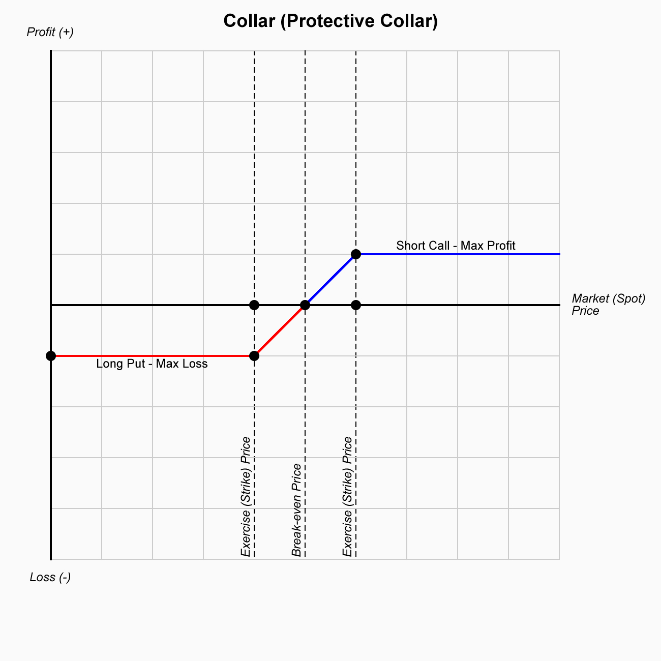
The collar strategy is used to limit downside risk while also capping upside potential. This strategy is suitable for investors who want to protect their gains or limit losses in a volatile or uncertain market but are willing to forgo unlimited potential profits in return for the protection provided by the put option.

Mechanics

The collar strategy typically involves the following steps:

Hold the Underlying Asset: The investor owns shares or an equivalent amount of the underlying asset (e.g., stocks, ETFs, etc.).
Sell a Covered Call: The investor sells a call option with a strike price higher than the current market price of the underlying asset. This allows them to collect a premium upfront, which can help offset the cost of purchasing the protective put.
Buy a Protective Put: The investor buys a put option with a strike price lower than the current market price. This limits the potential loss on the position if the price of the underlying asset falls significantly.

The protective collar limits both potential losses (through the protective put) and potential gains (through the sold call option). The cost of buying the protective put is partially or fully offset by the premium received from selling the call option, making it an affordable risk management strategy for some investors.

Example

Let’s consider an investor who owns 100 shares of a stock currently trading at $50 per share. The investor wants to limit potential losses but also wants to potentially profit from some upside movement. The investor decides to implement a collar strategy by selling a covered call and buying a protective put.

Hold the Underlying Asset: The investor holds 100 shares of the stock at $50 per share.
Sell a Covered Call: The investor sells a call option with a strike price of $55, expiring in one month, for a premium of $2 per share. The total premium received is $200 (since one options contract represents 100 shares).
Buy a Protective Put: The investor buys a put option with a strike price of $45, expiring in one month, for a premium of $1 per share. The total cost of the put option is $100.

In this case, the investor is using the $200 premium from the covered call to help offset the cost of the $100 premium for the protective put. Therefore, the net cost of the collar strategy is $100 ($200 premium from the call minus $100 cost of the put).

Possible Outcomes

If the stock price rises above $55:
- The investor will be obligated to sell the stock at $55 (due to the covered call). The stock is sold at the strike price of the call option.
- The profit from this scenario is limited to the difference between the initial stock price and the strike price of the call option, plus the premium received.
- For example, if the stock rises to $60, the investor sells the stock at $55, generating a $5 per share profit, plus the $2 premium from the call. The total profit is $7 per share.
If the stock price stays between $45 and $55:
- The put option expires worthless, and the investor keeps the stock. The call option also expires worthless, so the investor keeps the premium from the call ($200) but has no obligation to sell the stock.
- In this scenario, the investor’s effective profit is the premium received from selling the call ($200), minus the cost of the put ($100), for a net gain of $100.
If the stock price falls below $45:
- The put option is exercised, and the investor is able to sell the stock at $45 (the strike price of the put option).
- The maximum loss is limited to the difference between the current stock price and the put strike price, minus the premium received from the call. For example, if the stock falls to $40, the investor will sell it at $45, avoiding further losses below that price. The maximum loss would be $5 per share (from the initial price of $50 to the put strike price of $45), but this is offset by the $2 premium received from the call, so the net loss is $3 per share.

Risk/Reward Profile

Maximum Profit: The maximum profit in a collar strategy is limited to the strike price of the sold call (minus the purchase price of the stock) plus the premium received from selling the call. If the price of the underlying asset rises above the call strike price, the investor will be forced to sell the asset at the strike price, and any further price increases are not captured.
- Example: If the stock rises to $60, the maximum profit is $55 (strike price of the call) minus the $50 purchase price of the stock, plus the $2 premium received from the call, for a total maximum profit of $7 per share.
Maximum Loss: The maximum loss occurs if the price of the underlying asset falls below the strike price of the put, but the loss is capped at the difference between the stock’s current price and the put’s strike price (less the premium received from selling the call).
- Example: If the stock falls to $40, the maximum loss is $50 (purchase price of the stock) minus $45 (put strike price), plus the cost of the put premium ($100). This results in a maximum loss of $300 (or $3 per share), which is a limited loss compared to the potential loss without the collar.
Breakeven Point: The breakeven point occurs at the current price of the stock minus the premium received from the call option, plus the cost of the put option.
- Example: If the stock is at $50, the net premium received from the call is $200, and the cost of the put is $100. The breakeven point is $50 (current stock price) – $2 (call premium) + $1 (put premium) = $49 per share.

Pros

Downside Protection: The protective put provides downside protection, limiting potential losses if the price of the underlying asset falls sharply.
Income Generation: The premium received from selling the call option generates immediate income, which can help offset the cost of the put option or contribute to the overall return.
Defined Risk/Reward: The collar strategy provides a defined risk and defined reward. Investors know the maximum potential loss and gain upfront, which can help with risk management and planning.
Cost-Effective: In many cases, the premium received from selling the covered call can offset the cost of buying the protective put, making this strategy relatively inexpensive for the investor.

Cons

Limited Upside Potential: The collar strategy caps potential profits. If the underlying asset rises significantly above the call’s strike price, the investor will not benefit from the additional price increase. They are obligated to sell the asset at the strike price of the call option.
Opportunity Cost: While the investor has limited downside risk, the strategy also limits the upside potential, which could be frustrating if the underlying asset performs very well.
Complexity: The collar strategy can be more complex than simply holding the underlying asset, as it requires managing multiple options contracts (buying a put and selling a call) while maintaining a long position in the underlying asset.
Transaction Costs: There can be significant transaction costs associated with implementing the collar, especially when buying and selling options contracts frequently.

When to Use

Protect Gains: The collar is ideal for investors who have gained a substantial amount of value in an asset and want to lock in profits while still having limited exposure to downside risk.
Uncertain Market Conditions: This strategy is well-suited for times when the investor expects volatility in the market but is unsure of the direction. It provides a hedge against large losses while still allowing for some upside potential.
Neutral to Moderately Bullish: The investor believes that the asset’s price will stay within a specific range or rise moderately, but they want to limit losses if the price falls.

Conclusion

The collar (protective collar) strategy is a risk management tool that allows investors to protect against downside risk while capping potential upside gain. By combining a long position in the asset, selling a covered call, and buying a protective put, the collar provides a defined risk/reward profile. This strategy is useful for investors looking to hedge their positions in volatile markets, protect gains, or generate income through options premiums, while also being willing to limit potential profits. The strategy works well in markets with uncertainty or volatility and is especially attractive to investors with neutral to slightly bullish outlooks.

Admin

Financial Analysis, Financial Instruments

18 Jan 0

Cash-Secured Put

A Cash-Secured Put is an options trading strategy that involves selling a put option while setting aside sufficient cash to purchase the underlying asset (if the put option is exercised). This strategy is commonly used by investors who are willing to buy the underlying asset at a certain price (the strike price of the put) in exchange for receiving an upfront premium from selling the put option.

This strategy is considered conservative and is typically employed when an investor has a neutral to slightly bullish outlook on the underlying asset and is looking to generate income through premiums while potentially acquiring the asset at a price lower than its current market value.

Key Elements

Sell a Put Option: In this strategy, the investor sells a put option on a particular asset (like a stock, ETF, or index). By selling the put, the investor agrees to potentially buy the underlying asset at the strike price if the option is exercised by the buyer.
Set Aside Cash: The key characteristic of a cash-secured put is that the investor sets aside enough cash to purchase the underlying asset at the strike price if the put option is exercised. This ensures the investor can fulfill their obligation if the option is exercised.
Income Generation: By selling the put option, the investor receives a premium, which is the income generated from the strategy. The premium is kept regardless of whether the option is exercised, making this a potentially lucrative strategy when markets are flat or slightly bullish.
Neutral to Slightly Bullish Outlook: The investor typically has a neutral to slightly bullish outlook on the underlying asset. They may want to own the asset but are not willing to buy it at the current market price, so they are willing to potentially buy it at the lower strike price, collecting premium income in the process.

Objective

The main goal of a cash-secured put is to generate income from the premium received from selling the put option while keeping the possibility of acquiring the underlying asset at a discount (the strike price) if the option is exercised. It is used in scenarios where the investor is willing to buy the asset at the strike price but is also content with keeping the premium if the option expires worthless.

Mechanics

Sell a Put Option: The trader sells a put option with a specific strike price and expiration date. This obligates them to buy the underlying asset at the strike price if the put option is exercised by the buyer.
Set Aside Cash: The trader sets aside enough cash to purchase the underlying asset if the put is exercised. For example, if the strike price is $100 per share and the investor sells one put contract (which typically represents 100 shares), they must set aside $10,000 in cash to cover the purchase of 100 shares at the strike price.
Receive Premium: The trader receives the premium from selling the put option. This premium is theirs to keep, regardless of whether the option is exercised or expires worthless.
Expiration or Exercise:
- If the underlying asset price stays above the strike price: The put option expires worthless, and the investor keeps the premium as profit without having to buy the underlying asset.
- If the underlying asset price falls below the strike price: The put option is exercised, and the trader is obligated to buy the underlying asset at the strike price. In this case, the premium received from selling the put option helps to reduce the effective cost of acquiring the asset.

Maximum Profit

The maximum profit occurs when the put option expires worthless (i.e., the price of the underlying asset remains above the strike price). In this case, the investor keeps the full premium received for selling the put option as profit.

Mathematically:

Maximum Profit = Premium Received.

Maximum Loss

The maximum loss occurs if the price of the underlying asset falls to zero. In this case, the investor would have to buy the asset at the strike price, which would result in a significant loss. However, this loss is partially offset by the premium received from selling the put option.

Mathematically:

Maximum Loss = Strike Price of the Put – Premium Received (if the asset price falls to zero).

Breakeven Point

The breakeven point is the price at which the investor will neither make a profit nor a loss. It occurs when the price of the underlying asset is equal to the strike price minus the premium received.

Mathematically:

Breakeven = Strike Price – Premium Received.

Example

Let’s say an investor is interested in selling a cash-secured put on a stock currently trading at $50. The investor decides to sell a put option with a strike price of $45, expiring in one month, and receives a premium of $2 per share.

Sell the Put Option: The investor sells a put option with a strike price of $45, expiring in one month, for a premium of $2 per share.
Set Aside Cash: Since the strike price is $45, the investor must set aside enough cash to buy the stock at that price if the option is exercised. For one options contract (100 shares), this amounts to $4,500.
Premium Received: The investor collects $2 per share, or $200 (100 shares x $2).

Outcomes

If the stock stays above $45:
- The put option expires worthless, and the investor keeps the $200 premium as profit. The investor does not need to buy the stock.
If the stock falls to $40:
- The put option is exercised, and the investor is obligated to buy the stock at $45.
- The investor spends $4,500 to buy 100 shares of the stock at $45 each.
- The effective cost of the stock is reduced by the $200 premium, so the effective cost is $4,300 ($4,500 – $200 premium received).
- The investor now owns the stock at an average cost of $43 per share, even though the market price is $40 per share.
If the stock falls to $0:
- The investor is still obligated to buy the stock at $45, but now the stock is worth nothing.
- The loss is $4,500 (the total amount spent to buy the stock) minus the $200 premium received, resulting in a net loss of $4,300.

Risk/Reward Profile

Maximum Loss: The maximum loss occurs if the price of the underlying asset falls to zero, in which case the investor would incur a loss equal to the strike price minus the premium received. However, the loss is mitigated by the premium income.
- Maximum Loss = Strike Price – Premium Received (if the asset’s value drops to zero).
Maximum Profit: The maximum profit is limited to the premium received for selling the put option. The investor cannot earn more than the premium, even if the underlying asset’s price rises significantly.
- Maximum Profit = Premium Received.
Breakeven Point: The breakeven point is the price at which the net result of the strategy is zero, accounting for both the premium received and the price of the underlying asset.
- Breakeven = Strike Price – Premium Received.

When to Use

Neutral to Bullish Outlook: The investor expects the price of the underlying asset to either stay the same or increase slightly, but they are willing to buy the asset at the strike price if the market falls.
Generate Income: This strategy is ideal for generating income through premiums in a relatively stable or slightly bullish market. If the market remains above the strike price, the premium is a profitable outcome for the trader.
Willing to Acquire the Asset: This strategy is best suited for investors who are willing to own the underlying asset at a price lower than the current market price. The investor may view the potential acquisition as an opportunity to purchase the asset at a discounted price if the market price falls.

Pros

Income Generation: The premium received from selling the put option provides immediate income to the investor, which can be especially attractive in flat or slightly bullish markets.
Limited Risk: The risk is limited to the difference between the strike price and the premium received if the asset falls to zero. This makes it a relatively low-risk strategy when compared to strategies like selling naked puts or shorting the asset outright.
Potential Discounted Purchase: If the option is exercised, the investor can acquire the underlying asset at a discounted price (the strike price minus the premium).
Ideal for Neutral or Slightly Bullish Markets: This strategy works best when the investor believes the price of the asset will not fall below the strike price.

Cons

Limited Profit Potential: The maximum profit is capped at the premium received, so even if the underlying asset rises significantly, the investor will only profit from the premium.
Cash Requirement: The strategy requires the investor to set aside a significant amount of cash (equal to the strike price of the put multiplied by 100 shares per contract), which can tie up capital and reduce liquidity.
Risk of Ownership: If the price of the underlying asset falls below the strike price, the investor will have to buy the asset, and the value of that asset may continue to decline, leading to potential losses.
Missed Opportunity: If the market price stays above the strike price, the investor misses the opportunity to purchase the asset at a lower price, especially if the price drops after the option expires.

Example Summary

Stock Price: $50
Sell Put Option with Strike Price of $45
Premium Received: $2 per share
Set Aside Cash: $4,500 (for 100 shares)
Maximum Profit: $200 (premium received)
Maximum Loss: $4,300 (if the stock falls to zero)
Breakeven: $43 (strike price – premium received)

Conclusion

A cash-secured put is a relatively conservative strategy used to generate income through the premium received from selling put options, while also providing the opportunity to acquire the underlying asset at a discount if the option is exercised. The strategy is best suited for investors with a neutral to bullish outlook who are willing to own the asset at the strike price and are looking to generate income in a stable or slightly bullish market. The maximum risk is limited to the strike price of the put minus the premium received, and the maximum profit is limited to the premium received.

Admin

Financial Analysis, Financial Instruments

18 Jan 0

Cash-Backed Call (Cash-Secured Call)

A Cash-Secured Call (also known as a Cash-Backed Call) is a conservative options trading strategy that involves selling a covered call while having sufficient cash or liquid assets set aside to buy the underlying asset if the call is exercised. It’s similar to a covered call but instead of owning the underlying asset, the trader sets aside cash as collateral in case they need to buy the asset.

This strategy is typically used when the investor has a neutral to slightly bullish outlook on the underlying asset and aims to generate income from the premium received by selling the call option. The main difference between a cash-secured call and a standard covered call is that the cash-secured call does not require the investor to already own the underlying asset but instead uses cash to guarantee the potential purchase of the asset.

Key Elements

Sell a Call Option: The investor sells a call option on a stock, index, or other asset. This gives the buyer of the call the right, but not the obligation, to buy the underlying asset at the call’s strike price.
Cash Reserve: The investor sets aside enough cash to purchase the underlying asset if the option is exercised by the buyer. This amount should be equal to the strike price of the call option multiplied by the number of shares (or units of the asset) per contract (typically 100 shares per contract for stocks).
Neutral to Slightly Bullish Outlook: The investor sells the call option because they believe the asset’s price will either remain stable or increase slightly, but they don’t necessarily want to own the asset outright. They expect that the call will expire worthless or be exercised at a price higher than the market value.
Premium Income: By selling the call option, the investor collects a premium upfront, which represents the income from the strategy. This premium is kept regardless of whether the option is exercised.

Objective

The objective of a cash-secured call is to generate income through the premiums received from selling the call option while maintaining the ability to purchase the underlying asset if the call is exercised. It’s a neutral to slightly bullish strategy that allows an investor to earn money in a relatively flat or mildly rising market, without having to own the underlying asset in advance.

Mechanics

Sell a Call Option: The trader sells a call option with a specific strike price and expiration date. This obligates them to sell the underlying asset at the strike price if the buyer chooses to exercise the option.
Set Aside Cash: The trader sets aside cash equivalent to the strike price of the call option (multiplied by 100 for each options contract). This cash will be available to buy the underlying asset if the call option is exercised.
Receive Premium: The trader collects the premium from selling the call. This premium is theirs to keep whether or not the option is exercised.
Expiration or Exercise:
- If the underlying asset remains below the strike price: The call option expires worthless, and the investor keeps the premium as profit.
- If the underlying asset rises above the strike price: The buyer of the call may exercise the option, and the seller (the trader) will need to purchase the underlying asset at the current market price (if they don’t already own it) and sell it to the option holder at the strike price. The trader’s profit comes from the premium received plus any potential price appreciation up to the strike price.

Maximum Profit

The maximum profit in a cash-secured call strategy is limited to the premium received from selling the call option. Even if the price of the underlying asset rises significantly, the maximum profit is capped at the strike price plus the premium received.

Mathematically:

Maximum Profit = Premium Received + (Strike Price – Purchase Price) (if the trader already owns the underlying asset).

Maximum Loss

The maximum loss occurs if the price of the underlying asset falls to zero. This is because the trader still holds the cash-secured position but has no offsetting premium income (if the option expires worthless and the asset becomes worthless).

However, because the trader has set aside the cash to buy the asset, the maximum loss is limited to the full price of purchasing the underlying asset at the strike price (which would occur if the call is exercised).

Mathematically:

Maximum Loss = Amount Paid for Underlying Asset (if exercised at strike price and the asset’s value falls).

Breakeven Point

The breakeven point is the price at which the investor will not make a profit or loss from the strategy. It is calculated by taking the strike price of the call and subtracting the premium received from selling the call option.

Mathematically:

Breakeven = Strike Price of the Call – Premium Received.

Example

Let’s assume a stock is currently trading at $50, and you want to sell a cash-secured call on this stock:

Sell a Call Option: You sell a call option with a strike price of $55, expiring in one month, for a premium of $2 per share.
Set Aside Cash: Since the strike price is $55, you need to set aside $5,500 ($55 x 100 shares) in cash to cover the purchase of the stock if the option is exercised.
Premium Received: You collect $2 per share, so you receive $200 (100 shares x $2).

Outcomes

If the stock price stays below $55:
- The call option expires worthless, and you keep the $200 premium as profit. You don’t need to buy the stock.
If the stock price rises to $60:
- The call option is exercised, and you are obligated to sell the stock at $55.
- You will buy the stock at market price ($60) and sell it at $55.
- The net loss is the $5 difference in price minus the $200 premium received.
- In this case, the loss is mitigated by the premium received, but there is still a net loss because you had to buy at $60 and sell at $55.
If the stock price rises to $55:
- The option is exercised, and you sell the stock at $55. You effectively break even because you set aside $5,500 to purchase the stock, and the $200 premium received offsets the cost of the transaction.

Risk/Reward Profile

Maximum Loss: The maximum loss occurs if the price of the underlying asset drops to zero. This results in a complete loss of the value of the underlying asset, minus the premium received.
Maximum Profit: The maximum profit is limited to the premium received from selling the call, as the trader cannot earn more than the premium if the stock rises above the strike price.
Breakeven Point: The breakeven point is the strike price of the sold call minus the premium received.

When to Use

Neutral to Slightly Bullish Outlook: This strategy is used when the investor believes the price of the underlying asset will either remain stable or increase slightly. The premium received from selling the call provides income, and the strategy works well in a moderately bullish or flat market.
Income Generation: The strategy is ideal for income generation because it allows the investor to earn premium income by selling the call option. This is particularly useful when the investor is not expecting significant movement in the underlying asset and seeks additional income.
Limited Capital Risk: For investors who are hesitant to buy the underlying asset outright but still want to profit from slight upward movements, the cash-secured call offers a way to use cash as collateral instead of needing to buy the asset upfront.

Pros

Income Generation: The premium received from selling the call option provides immediate income, which is especially appealing in a neutral market.
Limited Risk: The strategy has limited risk, as the investor sets aside cash to buy the stock if necessary. However, the risk is limited to the decline in the stock’s value.
No Need to Own the Asset: Unlike a covered call, the investor does not need to own the asset upfront, as they are using cash as collateral.
Ideal for Sideways or Slightly Bullish Markets: This strategy works well in flat or mildly bullish markets where the stock price is not expected to rise dramatically above the strike price.

Cons

Limited Profit Potential: The maximum profit is capped at the premium received, meaning the investor cannot benefit from any price increase above the strike price.
Cash Requirement: The strategy requires the investor to set aside enough cash to purchase the underlying asset if the option is exercised, which can tie up a significant amount of capital.
Opportunity Cost: If the underlying asset rises above the strike price, the investor is forced to sell at the strike price, potentially missing out on higher gains.
Risk of Loss: If the underlying asset’s price falls significantly, the investor may incur a loss on the asset itself, although this loss can be offset by the premium received.

Example Summary

Stock Price: $50
Sell Call Option with a Strike Price of $55
Premium Received: $2 per share
Set

Aside Cash: $5,500 to buy the stock if exercised

Maximum Profit: $200 (premium received)
Maximum Loss: Limited to the amount paid to purchase the asset if the stock price falls to zero.
Breakeven: $53 (strike price of $55 – premium received)

Conclusion

A cash-secured call is a conservative options strategy that generates income through the premiums received from selling call options while setting aside cash to cover the potential purchase of the underlying asset if the option is exercised. It is best used in a neutral to slightly bullish market, where the investor expects little movement or slight appreciation in the asset’s price. The strategy offers limited risk, as the cash set aside can be used to purchase the asset if necessary, but the profit potential is capped at the premium received.

Admin

Financial Analysis, Financial Instruments

1 2 3 4 5

Financial Instruments

What is Mark-to-Market (MTM)?

The MTM Process in Futures Contracts

Key Features of Mark-to-Market

Why is Mark-to-Market Important?

Mark-to-Market Outside of Futures Contracts

Example of MTM in Action (Futures Contract)

Conclusion

Additional Forms of Risk Premiums

Key Points about Risk Premium

Example of Risk Premium

How Risk Premiums Affect Financial Markets

Risk Premium and the Unbiased Expectation Hypothesis (UEH)

Discreet Compounding

Continuous Compounding

Present Value (Discreet Compounding)

Pay-Off Diagram

Key Elements

Objectives

Mechanics

Example

Possible Outcomes

Risk/Reward Profile

Pros

Cons

When to Use

Conclusion

Key Elements

Objective

Mechanics

Maximum Profit

Risk/Reward Profile

When to Use

Conclusion

Key Elements

Objective

Mechanics

When to Use

Conclusion