Financial Analysis

Holding Period Return (HPR)

 

Holding Period Return (HPR)

Holding Period Return (HPR) is a measure of the total return on an investment over a specific period of time, regardless of whether the investment is held for a short or long duration. It takes into account both income earned from the investment (such as dividends or interest) and capital gains or losses due to price changes during the holding period.

HPR is particularly useful for assessing the performance of an investment over a discrete time period, like a year, month, or any other specified time frame. It’s often used in investment analysis to compare the performance of different assets, portfolios, or investment strategies.

 

---

Formula for Holding Period Return (HPR)

The basic formula for calculating the Holding Period Return (HPR) is:

 

$$\text{HPR} = \frac{\text{Ending Value} – \text{Beginning Value} + \text{Income}}{\text{Beginning Value}}$$

 

Where:

• Final Price: The final price of the investment at the end of the holding period.
• Original Price: The initial value of the investment at the start of the holding period.
• Income: Any income received during the holding period (such as dividends, interest, or other distributions).

 

---

Understanding the Components

• Original Price: This is the price at which the asset or security is initially purchased. For example, if you buy a stock at $100 per share, the beginning value is $100.
• Final Price: This is the price of the investment at the end of the holding period. For instance, if the stock price has risen to $120 by the end of the year, the ending value would be $120.
• Income: This includes any dividends, interest, or other distributions received during the holding period. For example, if the stock paid $5 in dividends over the year, this income would be added to the formula.

 

---

Examples of Holding Period Return (HPR)

Example 1: Stock Investment with Dividends

Suppose an investor buys 100 shares of a stock for $50 per share at the beginning of the year. During the year, the stock pays $2 per share in dividends, and by the end of the year, the stock price rises to $60 per share.

• Beginning Value = $50 × 100 shares = $5,000
• Ending Value = $60 × 100 shares = $6,000
• Income = $2 × 100 shares = $200 (dividends received)

Now, plug the values into the HPR formula:

 

$$\text{HPR} = \frac{6,000 – 5,000 + 200}{5,000} = \frac{1,200}{5,000} = 0.24 \text{ or } 24\%$$

 

In this case, the Holding Period Return is 24%, meaning the investor achieved a 24% return on the investment over the year, considering both capital appreciation and dividends.

 

Example 2: Bond Investment with Interest

Let’s assume an investor purchases a bond for $1,000. Over the next year, the bond pays $50 in interest (coupon payment), and the price of the bond rises to $1,050.

• Beginning Value = $1,000
• Ending Value = $1,050
• Income = $50 (interest received)

Now, apply the HPR formula:

 

$$\text{HPR} = \frac{1,050 – 1,000 + 50}{1,000} = \frac{100}{1,000} = 0.10 \text{ or } 10\%$$

 

In this case, the Holding Period Return is 10%.

 

---

Significance and Uses of Holding Period Return

The Holding Period Return is widely used for several reasons:

• Performance Evaluation: HPR helps investors assess how well their investments have performed over a given period, taking into account both price appreciation and income received.
• Comparison of Investments: Since HPR can be calculated for various types of investments (stocks, bonds, real estate, etc.), it allows for a direct comparison between different assets or portfolios to evaluate which has provided the better return over the same period.
• Risk-Adjusted Comparison: HPR can be used in conjunction with risk measures (like standard deviation or beta) to evaluate returns relative to the level of risk taken. This helps investors in decision-making by comparing not only returns but also the associated risks.
• Annualizing the Return: While HPR calculates the return for a specific holding period, it can be annualized to allow comparison between investments held for different lengths of time. This is particularly useful if investments are held for periods shorter or longer than one year.

 

---

Annualizing Holding Period Return (for non-annual periods)

When an investment is held for less than or more than a year, it is common to annualize the holding period return to make it comparable to annualized returns from other investments. The annualization process adjusts the return to reflect a full year, assuming the investment’s performance over the holding period would continue at the same rate.

To annualize a return, you can use the following formula:

 

$$\text{Annualized HPR} = \left(1 + \text{HPR}\right)^{\frac{1}{n}} – 1$$

 

Where:

• HPR is the holding period return for the investment.
• n is the number of years (or fractions of a year) the investment was held.

 

Example: Annualizing a Six-Month Return

Let’s say an investor has a holding period return of 10% for an investment held for 6 months. To annualize the return, use the formula:

 

$$\text{Annualized HPR} = (1 + 0.10)^{\frac{1}{0.5}} – 1 = 1.10^2 – 1 = 1.21 – 1 = 0.21 \text{ or } 21\%$$

 

In this example, the annualized holding period return is 21%, assuming the same performance would continue for the full year.

 

---

Limitations of Holding Period Return

While HPR is a useful measure, it has some limitations:

• Does Not Account for Compounding: If the investment involves reinvestment of income (such as dividends or interest), HPR does not account for the compounding effect unless the income is reinvested during the holding period.
• Non-Standardized Time Frame: Since the holding period can vary significantly (from days to years), HPR doesn’t provide a standardized way to compare investments over different time periods unless the return is annualized.
• Does Not Factor in Risk: HPR focuses on the return of an investment but does not directly measure the risk taken to achieve that return. It can be misleading when comparing investments with different risk profiles.
• Excludes Transaction Costs: The formula assumes no transaction costs (such as brokerage fees), taxes, or other expenses, which could affect the net return.

 

---

Real-World Application of HPR

HPR is often used in the following scenarios:

• Equity and Fixed Income Investment Performance: Investors and portfolio managers use HPR to assess the return on stocks, bonds, or mutual funds over a specific period, including dividends, interest, and capital gains.
• Real Estate Investments: HPR can be used to calculate the total return on real estate investments, considering both rental income and changes in property value.
• Private Equity: HPR is often applied to investments in private equity, where investors want to evaluate the overall return over the period they held the investment, factoring in distributions and changes in value.

 

---

Conclusion

The Holding Period Return (HPR) is an essential metric for measuring the total return of an investment over a specific period. By including both income and capital gains or losses, HPR provides a comprehensive picture of an investment’s performance. While HPR is a simple and effective tool for performance assessment, investors should be aware of its limitations, including its lack of consideration for compounding, risk, and transaction costs. Annualizing the return can make it more comparable to other investments held over different periods. HPR remains a fundamental calculation for comparing the performance of various assets and for evaluating the success of investment strategies.

 

---

Formula

 

$$\begin{aligned} HPR\; &= \left [ Final\;Price\;-\;Original\;Price\;+\;Income \over Original\;Price \right ] \\\\ &= \;\left [ Capital\;Gain\;+\;Dividends \over Original\;Price \right ] \end{aligned}$$

 

---

Holding Period Return (HPR)

 

 

Compound Interest

 

Market Capitalisation

Beta Coefficient (β)

Notes

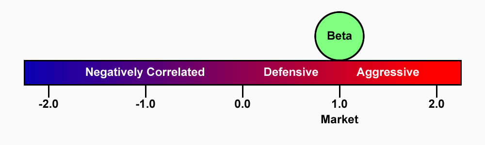
The Beta Coefficient measures the volatility of a particular share (systematic risk) in comparison to the market (unsystematic risk). It describes the sensitivity of a security’s returns in response to swings in the market.

Systematic risk is the underlying risk that affects the entire market. Large changes in macroeconomic variables, such as interest rates, inflation, GDP, or foreign exchange, are changes that impact the broader market and that cannot be avoided through diversification. The Beta coefficient relates ‘the market’ systematic risk to ‘stock-specific’ unsystematic risk by comparing the rate of change between ‘the market’ and ‘stock-specific’ returns.

Statistically, beta represents the slope of the line through a regression of data points from an individual stock’s returns against those of the market.

The beta calculation is used to help investors understand whether a stock moves in the same direction as the rest of the market, and how volatile or risky it is compared to the market.

For beta to provide any insight, the ‘market’ used as a benchmark should be related to the stock.

For example, calculating a bond ETF’s beta by using the S&P 500 as the benchmark isn’t helpful because bonds and stocks are too dissimilar. The benchmark or market return used in the calculation needs to be related to the stock because an investor is trying to gauge how much risk a stock is adding to a portfolio.

A stock that deviates very little from the market doesn’t add a lot of risk to a portfolio, but it also doesn’t increase the theoretical potential for greater returns.

 

The beta of the market portfolio is always 1.0

• β = 1.0  (The security has the same volatility as the market as a whole.)
• β > 1.0  (Aggressive investment with volatility of returns greater than the market.)
• β < 1.0  (Defensive investment with volatility of returns less than the market.)
• β < 0.0  (An investment with returns that are negatively correlated with the returns of the market.)

 

 

---

Formula

 

$$  Beta\;Coefficient\;(β)  = \left [Covariance (rp, rb) \over Variance (rb) \right ]$$

 

---

Beta Coefficient

 

Sharpe Ratio (Reward-to-Volatility)

 

The Sharpe Ratio is a widely used measure to assess the risk-adjusted return of an investment or portfolio. It helps investors understand how well the return of an asset compensates for the risk taken to achieve that return. The Sharpe Ratio is named after William F. Sharpe, who developed it in 1966.

 

---

Purpose

The Sharpe Ratio allows investors to evaluate whether an investment’s returns are due to smart investment decisions or excessive risk-taking. A higher Sharpe Ratio indicates better risk-adjusted returns, meaning the investor is receiving more return per unit of risk. Conversely, a lower Sharpe Ratio suggests that the return isn’t compensating the investor adequately for the level of risk being taken.

 

---

Formula

The Sharpe Ratio is calculated as:

$$S = \frac{R_p – R_f}{\sigma_p}$$

 

Where:

• 
  $S$ 

  = Sharpe Ratio

• 
  $R_p$ 

  = Return of the portfolio or investment (often the expected return or the actual return over a specific period)

• 
  $R_f$ 

  = Risk-free rate (the return on a risk-free investment, typically a government bond like U.S. Treasuries)

• 
  $\sigma_p$ 

  = Standard deviation of the portfolio’s returns, a measure of risk (volatility)

 

---

Breakdown of the Formula

1. 
   $R_p – R_f$ 

   :

   • This represents the excess return or risk premium. It’s the return earned by the investment over and above the return on a risk-free asset. The risk-free rate is used as a benchmark, as it represents an investment with no risk. The higher the excess return, the more attractive the investment appears.
2. 
   $\sigma_p$ 

   :

   • This is the standard deviation of the portfolio’s returns, which measures the volatility or risk associated with the investment. A higher standard deviation means greater fluctuations in returns, indicating higher risk. In essence, it tells how spread out the investment’s returns are, with greater variability implying higher risk.

 

---

Interpretation

• Sharpe Ratio > 1: The investment is considered to have good risk-adjusted returns. The higher the ratio, the better the risk-return tradeoff.
• Sharpe Ratio = 1: The investment has a moderate risk-adjusted return. It means the return justifies the risk taken.
• Sharpe Ratio < 1: The investment is considered to have poor risk-adjusted returns. The returns are not compensating adequately for the risk.
• Sharpe Ratio = 0: The return is exactly the same as the risk-free rate, so the investor is not earning any additional return for the risk.
• Negative Sharpe Ratio: This suggests that the investment has underperformed the risk-free rate, indicating that the investor would have been better off investing in a risk-free asset.

 

Example

Let’s say you have the following data:

• Portfolio return (
  $R_p$ 

  ): 10% (0.10)

• Risk-free rate (
  $R_f$ 

  ): 2% (0.02)

• Portfolio’s standard deviation (
  $\sigma_p$ 

  ): 15% (0.15)

The Sharpe Ratio would be calculated as:

$$S = \frac{0.10 – 0.02}{0.15} = \frac{0.08}{0.15} = 0.533$$

 

This means the Sharpe Ratio for this investment is 0.533, which indicates that the investment provides less return than its risk would ideally warrant (i.e., the risk-adjusted return is moderate).

 

---

What Does the Sharpe Ratio Tell You?

1. Risk-Adjusted Return: The Sharpe Ratio helps you assess how much return you are getting per unit of risk. In the example above, a ratio of 0.533 means that for each unit of risk, you are getting only a fraction of a unit of return. Investors typically want to see higher ratios, which indicate a more favorable return relative to the risk taken.
2. Comparison of Different Investments: The Sharpe Ratio is very useful when comparing different investments or portfolios. It helps investors determine which investment offers the best return for the least amount of risk. For example, an investor might compare two portfolios with similar returns but different risks. The portfolio with the higher Sharpe Ratio would be considered more efficient, as it achieves that return with less risk.
3. Performance Evaluation: For portfolio managers or fund managers, the Sharpe Ratio is an important tool for evaluating the performance of a fund. A higher Sharpe Ratio suggests the manager is generating more return relative to the risk they are taking on.

 

---

Limitations

1. Assumes Normal Distribution of Returns: The Sharpe Ratio assumes that returns are normally distributed (i.e., they follow a bell curve). However, financial returns can be skewed or exhibit “fat tails” (extreme events), making the Sharpe Ratio less reliable during periods of market stress or unusual events.
2. Does Not Account for All Risks: The Sharpe Ratio mainly focuses on volatility as a measure of risk, but it doesn’t account for other types of risks like liquidity risk, credit risk, or event risk. Therefore, it may not give a complete picture of an investment’s risk profile.
3. Doesn’t Handle Negative Returns Well: If an investment has consistently negative returns, the Sharpe Ratio can become misleading, as it might suggest a positive risk-adjusted return even though the investor is losing money.
4. Risk-Free Rate Assumption: The choice of the risk-free rate is subjective and can affect the Sharpe Ratio. For example, using U.S. Treasury bonds as the risk-free asset may not be appropriate in all countries or scenarios.

 

---

Sharpe Ratio vs. Other Risk-Adjusted Return Metrics

1. Sortino Ratio: Unlike the Sharpe Ratio, which uses total volatility, the Sortino Ratio only considers downside volatility (the risk of negative returns). This makes it more useful when an investor is concerned only about the risk of losses.
2. Treynor Ratio: The Treynor Ratio is similar to the Sharpe Ratio but uses beta (a measure of market risk) instead of standard deviation. It focuses on how well a portfolio performs relative to its exposure to systematic (market) risk rather than total volatility.

 

---

Conclusion

The Sharpe Ratio is a valuable tool for investors to assess the return on an investment relative to the risk taken. A higher Sharpe Ratio indicates a more favorable risk-adjusted return, while a lower ratio suggests the investment is not compensating adequately for the risk. However, it’s important to be aware of its limitations and use it in conjunction with other metrics to get a more complete picture of an investment’s risk and return characteristics.

 

---

Formula

$$\begin{aligned} Sharpe\;Ratio &=  \left[ Expected\;Return\;-\;Risk\;Free\;Rate\over Standard\;Deviation\;of\;Excess\;Return \right] \\\\\\\ &=  \left[ Risk\;Premium\over Standard\;Deviation\;of\;Excess\;Return \right] \\\\\\\ &= \left [E(r_i)\;-\;r_f \over \sigma_i \right]\end{aligned}$$

 

---

Graph

 

---

Sharpe Ratio

 

---

Sharpe Ratio